py_eddy_tracker.dataset.grid.RegularGridDataset¶

class py_eddy_tracker.dataset.grid.RegularGridDataset(*args, **kwargs)[source]¶

Bases: GridDataset

Class only for regular grid

Parameters:

filename (str) – Filename to load
x_name (str) – Name of longitude coordinates
y_name (str) – Name of latitude coordinates
centered (bool,None) – Allow to know how coordinates could be used with pixel
indexs (dict) – A dictionary that sets indexes to use for non-coordinate dimensions
unset (bool) – Set to True to create an empty grid object without file
nan_masking (bool) – Set to True to replace data.mask with isnan method result

Methods

`add_grid`	Add a grid in handler
`add_uv`	Compute a u and v grid
`add_uv_lagerloef`
`advect`	At each call it will update position in place with u & v field
`bbox_indice`
`bessel_band_filter`
`bessel_high_filter`
`bessel_low_filter`
`c_to_bounds`	Centered coordinates to bounds coordinates
`check_order`
`clean`
`clean_land`	Function to remove all land pixel
`compute_finite_difference`
`compute_pixel_path`	Give a series of indexes describing the path between two positions
`compute_stencil`	Apply stencil ponderation on field.
`contour`
`convolve_filter_with_dynamic_kernel`
`copy`	Duplicate the variable from grid_in in grid_out
`display`
`eddy_identification`	Compute eddy identification on the specified grid
`estimate_kernel_shape`
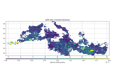
`filament`	Produce filament with concatenation of advection
`finalize_kernel`
`get_amplitude`
`get_mask`
`get_pixels_in`	Get indexes of pixels in contour.
`get_step_in_km`
`get_uavg`	Compute geostrophic speed around successive contours Returns the average
`grid`	Give the grid required
`grid_tiles`	Give the grid tiles required, without buffer system
`high_filter`	Return the high-pass filtered grid, by substracting to the initial grid the low-pass filtered grid (default: order=1)
`init_speed_coef`	Draft
`interp`	Compute z over lons, lats
`is_circular`	Check if the grid is circular
`kernel_bessel`	wave_length in km order must be int
`kernel_lanczos`	Not really operational wave_length in km order must be int
`kernel_loess`	https://fr.wikipedia.org/wiki/R%C3%A9gression_locale
`lanczos_high_filter`
`lanczos_low_filter`
`load`	Load variable (data).
`load_general_features`	Load attrs to be stored in object
`low_filter`	Return the low-pass filtered grid (default: order=1)
`nearest_grd_indice`
`normalize_x_indice`
`populate`
`regrid`	Interpolate another grid at the current grid position
`setup_coordinates`
`spectrum_lonlat`
`speed_coef_mean`	Some nan can be computed over contour if we are near borders, something to explore
`units`	Get unit from variable
`uv_for_advection`	Get U,V to be used in degrees with precomputed time step
`with_array`	Geo matrix data must be ordered like this (X,Y) and masked with numpy.ma.array
`write`	Write dataset output with same format as input

Attributes

`x_size`
`EARTH_RADIUS`
`GRAVITY`
`N`
`bounds`	Give bounds
`centered`
`contours`
`coordinates`
`dimensions`
`filename`
`global_attrs`
`indexs`
`is_centered`	Give True if pixel is described with its center's position or a corner
`nan_mask`
`variables`
`variables_description`
`vars`
`x_bounds`
`x_c`
`x_dim`
`xstep`	Only for regular grid with no step variation
`y_bounds`
`y_c`
`y_dim`
`ystep`	Only for regular grid with no step variation

add_uv(grid_height, uname='u', vname='v', stencil_halfwidth=4)[source]¶

Compute a u and v grid

Parameters:

grid_height (str) – grid name where the funtion will apply stencil method
uname (str) – future name of u
vname (str) – future name of v
stencil_halfwidth (int) – largest stencil could be apply (max: 4)

\[ \begin{align}\begin{aligned}u = \frac{g}{f} \frac{dh}{dy}\\v = -\frac{g}{f} \frac{dh}{dx}\end{aligned}\end{align} \]

where

\[ \begin{align}\begin{aligned}g = gravity\\f = 2 \Omega sin(\phi)\end{aligned}\end{align} \]

Eddy detection : Med

Eddy detection : Antartic Circumpolar Current

Eddy detection : Gulf stream

Eddy detection and filter

Get mean of grid in each eddies

Eddy detection on SLA and ADT

Grid advection

LAVD experiment

Collocating external data

add_uv_lagerloef(grid_height, uname='u', vname='v', schema=15, **kwargs)[source]¶

advect(x, y, u_name, v_name, nb_step=10, rk4=True, **kw)[source]¶

At each call it will update position in place with u & v field

It’s a dummy advection using only one layer of current

Parameters:

x (array) – Longitude of obs to move
y (array) – Latitude of obs to move
u_name (str,array) – U field to advect obs
v_name (str,array) – V field to advect obs
nb_step (int) – Number of iterations before releasing data

Grid advection

LAVD experiment

LAVD detection and geometric detection

bbox_indice(vertices)[source]¶

bessel_band_filter(grid_name, wave_length_inf, wave_length_sup, **kwargs)[source]¶

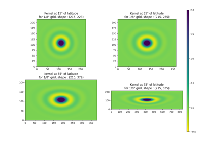
bessel_high_filter(grid_name, wave_length, order=1, lat_max=85, **kwargs)[source]¶

Parameters:

grid_name (str) – grid to filter, data will replace original one
wave_length (float) – in km
order (int) – order to use, if > 1 negative values of the cardinal sinus are present in kernel
lat_max (float) – absolute latitude, no filtering above
kwargs (dict) – look at RegularGridDataset.convolve_filter_with_dynamic_kernel()

Eddy detection : Med

Eddy detection : Antartic Circumpolar Current

Eddy detection : Gulf stream

Eddy detection and filter

Eddy detection on SLA and ADT

Grid filtering in PET

LAVD detection and geometric detection

Collocating external data

bessel_low_filter(grid_name, wave_length, order=1, lat_max=85, **kwargs)[source]¶

static check_order(order)[source]¶

clean_land(name)[source]¶: Function to remove all land pixel

compute_finite_difference(data, schema=1, mode='reflect', vertical=False, second=False)[source]¶

compute_pixel_path(x0, y0, x1, y1)[source]¶: Give a series of indexes describing the path between two positions

compute_stencil(data, stencil_halfwidth=4, mode='reflect', vertical=False)[source]¶

Apply stencil ponderation on field.

Parameters:

data (array) – array where apply stencil
stencil_halfwidth (int) – from 1 t0 4, maximal stencil used
mode (str) – convolution mode
vertical (bool) – if True, method apply a vertical convolution

Returns:

gradient array from stencil application

Return type:

array

Short story, how to get stencil coefficient for stencil (3 points, 5 points and 7 points)

Taylor’s theorem:

\[f(x \pm h) = f(x) \pm f'(x)h + \frac{f''(x)h^2}{2!} \pm \frac{f^{(3)}(x)h^3}{3!} + \frac{f^{(4)}(x)h^4}{4!} \pm \frac{f^{(5)}(x)h^5}{5!} + O(h^6)\]

If we stop at O(h^2), we get classic differenciation (stencil 3 points):

\[f(x+h) - f(x-h) = f(x) - f(x) + 2 f'(x)h + O(h^2)\]

\[f'(x) = \frac{f(x+h) - f(x-h)}{2h} + O(h^2)\]

If we stop at O(h^4), we will get stencil 5 points:

(1)¶\[f(x+h) - f(x-h) = 2 f'(x)h + 2 \frac{f^{(3)}(x)h^3}{3!} + O(h^4)\]

(2)¶\[f(x+2h) - f(x-2h) = 4 f'(x)h + 16 \frac{f^{(3)}(x)h^3}{3!} + O(h^4)\]

If we multiply equation (1) by 8 and substract equation (2), we get:

\[8(f(x+h) - f(x-h)) - (f(x+2h) - f(x-2h)) = 16 f'(x)h - 4 f'(x)h + O(h^4)\]

\[f'(x) = \frac{f(x-2h) - 8f(x-h) + 8f(x+h) - f(x+2h)}{12h} + O(h^4)\]

If we stop at O(h^6), we will get stencil 7 points:

(3)¶\[f(x+h) - f(x-h) = 2 f'(x)h + 2 \frac{f^{(3)}(x)h^3}{3!} + 2 \frac{f^{(5)}(x)h^5}{5!} + O(h^6)\]

(4)¶\[f(x+2h) - f(x-2h) = 4 f'(x)h + 16 \frac{f^{(3)}(x)h^3}{3!} + 64 \frac{f^{(5)}(x)h^5}{5!} + O(h^6)\]

(5)¶\[f(x+3h) - f(x-3h) = 6 f'(x)h + 54 \frac{f^{(3)}(x)h^3}{3!} + 486 \frac{f^{(5)}(x)h^5}{5!} + O(h^6)\]

If we multiply equation (3) by 45 and substract equation (4) multiply by 9 and add equation (5), we get:

\[45(f(x+h) - f(x-h)) - 9(f(x+2h) - f(x-2h)) + (f(x+3h) - f(x-3h)) = 90 f'(x)h - 36 f'(x)h + 6 f'(x)h + O(h^6)\]

\[f'(x) = \frac{-f(x-3h) + 9f(x-2h) - 45f(x-h) + 45f(x+h) - 9f(x+2h) +f(x+3h)}{60h} + O(h^6)\]

…

contour(ax, name, factor=1, ref=None, **kwargs)[source]¶

Parameters:

ax (matplotlib.axes.Axes) – matplotlib axes used to draw
name (str,array) – variable to display, could be an array
factor (float) – multiply grid by
ref (float,None) – if defined, all coordinates are wrapped with ref as western boundary
kwargs (dict) – look at matplotlib.axes.Axes.contour()

convolve_filter_with_dynamic_kernel(grid, kernel_func, lat_max=85, extend=False, **kwargs_func)[source]¶

Parameters:

grid (str) – grid name
kernel_func (func) – function of kernel to use
lat_max (float) – absolute latitude above no filtering apply
extend (bool) – if False, only non masked value will return a filtered value
kwargs_func (dict) – look at kernel_func

Returns:

filtered value

Return type:

array

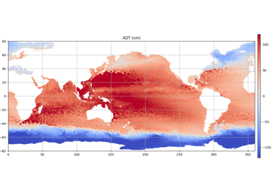
display(ax, name, factor=1, ref=None, **kwargs)[source]¶

Parameters:

ax (matplotlib.axes.Axes) – matplotlib axes used to draw
name (str,array) – variable to display, could be an array
factor (float) – multiply grid by
ref (float,None) – if defined, all coordinates are wrapped with ref as western boundary
kwargs (dict) – look at matplotlib.axes.Axes.pcolormesh()

Eddy detection : Med

Eddy detection : Antartic Circumpolar Current

Eddy detection : Gulf stream

Eddy detection and filter

Get mean of grid in each eddies

Eddy detection on SLA and ADT

Stastics on identification files

Grid filtering in PET

Select pixel in eddies

LAVD experiment

Get Okubo Weis

FSLE experiment in med

LAVD detection and geometric detection

Birth and death

Count center

Geographical statistics

Count pixel used

Collocating external data

Network Analysis

estimate_kernel_shape(lat, wave_length, order)[source]¶

filament(x, y, u_name, v_name, nb_step=10, filament_size=6, rk4=True, **kw)[source]¶

Produce filament with concatenation of advection

It’s a dummy advection using only one layer of current

Parameters:

x (array) – Longitude of obs to move
y (array) – Latitude of obs to move
u_name (str,array) – U field to advect obs
v_name (str,array) – V field to advect obs
nb_step (int) – Number of iteration before releasing data
filament_size (int) – Number of point by filament

Returns:

x,y for a line

Grid advection

finalize_kernel(kernel, order, half_x_pt, half_y_pt)[source]¶

get_pixels_in(contour)[source]¶

Get indexes of pixels in contour.

Parameters:: contour (vertice,Path) – Contour that encloses some pixels
Returns:: Indexes of grid in contour
Return type:: array[int],array[int]

get_step_in_km(lat, wave_length)[source]¶

init_speed_coef(uname='u', vname='v')[source]¶: Draft

interp(grid_name, lons, lats, method='bilinear')[source]¶

Compute z over lons, lats

Parameters:

grid_name (str) – Grid to be interpolated
lons – new x
lats – new y
method (str) – Could be ‘bilinear’ or ‘nearest’

Returns:

new z

is_circular()[source]¶: Check if the grid is circular

kernel_bessel(lat, wave_length, order=1)[source]¶: wave_length in km order must be int

kernel_lanczos(lat, wave_length, order=1)[source]¶: Not really operational wave_length in km order must be int

kernel_loess(lat, wave_length, order=1)[source]¶: https://fr.wikipedia.org/wiki/R%C3%A9gression_locale

lanczos_high_filter(grid_name, wave_length, order=1, lat_max=85, **kwargs)[source]¶

lanczos_low_filter(grid_name, wave_length, order=1, lat_max=85, **kwargs)[source]¶

nearest_grd_indice(x, y)[source]¶

normalize_x_indice(indices)[source]¶

regrid(other, grid_name, new_name=None)[source]¶

Interpolate another grid at the current grid position

Parameters:

other (RegularGridDataset)
grid_name (str) – variable name to interpolate
new_name (str) – name used to store, if None method will use current ont

Collocating external data

setup_coordinates()[source]¶

spectrum_lonlat(grid_name, area=None, ref=None, **kwargs)[source]¶

speed_coef_mean(contour)[source]¶: Some nan can be computed over contour if we are near borders, something to explore

uv_for_advection(u_name=None, v_name=None, time_step=600, h_name=None, backward=False, factor=1)[source]¶

Get U,V to be used in degrees with precomputed time step

Parameters:

u_name (None,str,array) – U field to advect obs, if h_name is None
v_name (None,str,array) – V field to advect obs, if h_name is None
h_name (None,str,array) – H field to compute UV to advect obs, if u_name and v_name are None
time_step (int) – Number of second for each advection

classmethod with_array(coordinates, datas, variables_description=None, **kwargs)[source]¶: Geo matrix data must be ordered like this (X,Y) and masked with numpy.ma.array

x_size¶

property xstep¶: Only for regular grid with no step variation

property ystep¶: Only for regular grid with no step variation