Grid advection

Dummy advection which use only static geostrophic current, which didn’t solve the complex circulation of the ocean.

import re

from matplotlib import pyplot as plt
from matplotlib.animation import FuncAnimation
from numpy import arange, isnan, meshgrid, ones

from py_eddy_tracker.data import get_demo_path
from py_eddy_tracker.dataset.grid import RegularGridDataset
from py_eddy_tracker.gui import GUI_AXES
from py_eddy_tracker.observations.observation import EddiesObservations

Load Input grid ADT

g = RegularGridDataset(
    get_demo_path("dt_med_allsat_phy_l4_20160515_20190101.nc"), "longitude", "latitude"
)
# Compute u/v from height
g.add_uv("adt")

Load detection files

a = EddiesObservations.load_file(get_demo_path("Anticyclonic_20160515.nc"))
c = EddiesObservations.load_file(get_demo_path("Cyclonic_20160515.nc"))

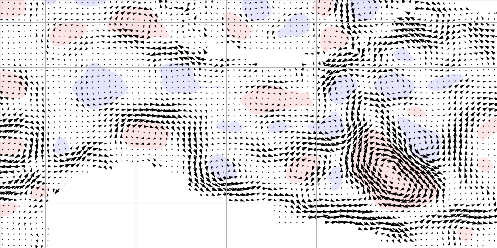
Quiver from u/v with eddies

fig = plt.figure(figsize=(10, 5))
ax = fig.add_axes([0, 0, 1, 1], projection=GUI_AXES)
ax.set_xlim(19, 30), ax.set_ylim(31, 36.5), ax.grid()
x, y = meshgrid(g.x_c, g.y_c)
a.filled(ax, facecolors="r", alpha=0.1), c.filled(ax, facecolors="b", alpha=0.1)
_ = ax.quiver(x.T, y.T, g.grid("u"), g.grid("v"), scale=20)

class VideoAnimation(FuncAnimation):
    def _repr_html_(self, *args, **kwargs):
        """To get video in html and have a player"""
        content = self.to_html5_video()
        return re.sub(
            r'width="[0-9]*"\sheight="[0-9]*"', 'width="100%" height="100%"', content
        )

    def save(self, *args, **kwargs):
        if args[0].endswith("gif"):
            # In this case gif is used to create thumbnail which is not used but consume same time than video
            # So we create an empty file, to save time
            with open(args[0], "w") as _:
                pass
            return
        return super().save(*args, **kwargs)

Anim

Particles setup

step_p = 1 / 8
x, y = meshgrid(arange(13, 36, step_p), arange(28, 40, step_p))
x, y = x.reshape(-1), y.reshape(-1)
# Remove all original position that we can't advect at first place
m = ~isnan(g.interp("u", x, y))
x0, y0 = x[m], y[m]
x, y = x0.copy(), y0.copy()

Movie properties

kwargs = dict(frames=arange(51), interval=100)
kw_p = dict(u_name="u", v_name="v", nb_step=2, time_step=21600)
frame_t = kw_p["nb_step"] * kw_p["time_step"] / 86400.0

Function

def anim_ax(**kw):
    t = 0
    fig = plt.figure(figsize=(10, 5), dpi=55)
    axes = fig.add_axes([0, 0, 1, 1], projection=GUI_AXES)
    axes.set_xlim(19, 30), axes.set_ylim(31, 36.5), axes.grid()
    a.filled(axes, facecolors="r", alpha=0.1), c.filled(axes, facecolors="b", alpha=0.1)
    line = axes.plot([], [], "k", **kw)[0]
    return fig, axes.text(21, 32.1, ""), line, t


def update(i_frame, t_step):
    global t
    x, y = p.__next__()
    t += t_step
    l.set_data(x, y)
    txt.set_text(f"T0 + {t:.1f} days")

Filament forward

Draw 3 last position in one path for each particles., it could be run backward with backward=True option in filament method

p = g.filament(x, y, **kw_p, filament_size=3)
fig, txt, l, t = anim_ax(lw=0.5)
_ = VideoAnimation(fig, update, **kwargs, fargs=(frame_t,))

Particle forward

Forward advection of particles

p = g.advect(x, y, **kw_p)
fig, txt, l, t = anim_ax(ls="", marker=".", markersize=1)
_ = VideoAnimation(fig, update, **kwargs, fargs=(frame_t,))

We get last position and run backward until original position

p = g.advect(x, y, **kw_p, backward=True)
fig, txt, l, _ = anim_ax(ls="", marker=".", markersize=1)
_ = VideoAnimation(fig, update, **kwargs, fargs=(-frame_t,))

Particles stat

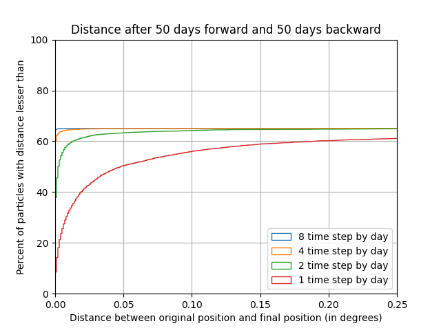
Time_step settings

Dummy experiment to test advection precision, we run particles 50 days forward and backward with different time step and we measure distance between new positions and original positions.

fig = plt.figure()
ax = fig.add_subplot(111)
kw = dict(
    bins=arange(0, 50, 0.001),
    cumulative=True,
    weights=ones(x0.shape) / x0.shape[0] * 100.0,
    histtype="step",
)
for time_step in (10800, 21600, 43200, 86400):
    x, y = x0.copy(), y0.copy()
    kw_advect = dict(
        nb_step=int(50 * 86400 / time_step), time_step=time_step, u_name="u", v_name="v"
    )
    g.advect(x, y, **kw_advect).__next__()
    g.advect(x, y, **kw_advect, backward=True).__next__()
    d = ((x - x0) ** 2 + (y - y0) ** 2) ** 0.5
    ax.hist(d, **kw, label=f"{86400. / time_step:.0f} time step by day")
ax.set_xlim(0, 0.25), ax.set_ylim(0, 100), ax.legend(loc="lower right"), ax.grid()
ax.set_title("Distance after 50 days forward and 50 days backward")
ax.set_xlabel("Distance between original position and final position (in degrees)")
_ = ax.set_ylabel("Percent of particles with distance lesser than")

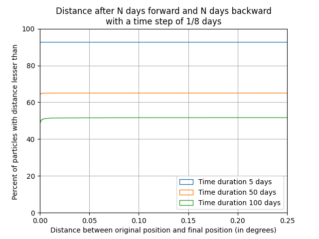
Time duration

We keep same time_step but change time duration

fig = plt.figure()
ax = fig.add_subplot(111)
time_step = 10800
for duration in (5, 50, 100):
    x, y = x0.copy(), y0.copy()
    kw_advect = dict(
        nb_step=int(duration * 86400 / time_step),
        time_step=time_step,
        u_name="u",
        v_name="v",
    )
    g.advect(x, y, **kw_advect).__next__()
    g.advect(x, y, **kw_advect, backward=True).__next__()
    d = ((x - x0) ** 2 + (y - y0) ** 2) ** 0.5
    ax.hist(d, **kw, label=f"Time duration {duration} days")
ax.set_xlim(0, 0.25), ax.set_ylim(0, 100), ax.legend(loc="lower right"), ax.grid()
ax.set_title(
    "Distance after N days forward and N days backward\nwith a time step of 1/8 days"
)
ax.set_xlabel("Distance between original position and final position (in degrees)")
_ = ax.set_ylabel("Percent of particles with distance lesser than ")