LAVD experiment

Naive method to reproduce LAVD(Lagrangian-Averaged Vorticity deviation) method with a static velocity field. In the current example we didn’t remove a mean vorticity.

Method are described here:

• Abernathey, Ryan, and George Haller. “Transport by Lagrangian Vortices in the Eastern Pacific”, Journal of Physical Oceanography 48, 3 (2018): 667-685, accessed Feb 16, 2021, https://doi.org/10.1175/JPO-D-17-0102.1

• Transport by Coherent Lagrangian Vortices, R. Abernathey, Sinha A., Tarshish N., Liu T., Zhang C., Haller G., 2019, Talk a t the Sources and Sinks of Ocean Mesoscale Eddy Energy CLIVAR Workshop

import re

from matplotlib import pyplot as plt
from matplotlib.animation import FuncAnimation
from numpy import arange, meshgrid, zeros

from py_eddy_tracker.data import get_demo_path
from py_eddy_tracker.dataset.grid import RegularGridDataset
from py_eddy_tracker.gui import GUI_AXES
from py_eddy_tracker.observations.observation import EddiesObservations

def start_ax(title="", dpi=90):
    fig = plt.figure(figsize=(16, 9), dpi=dpi)
    ax = fig.add_axes([0, 0, 1, 1], projection=GUI_AXES)
    ax.set_xlim(0, 32), ax.set_ylim(28, 46)
    ax.set_title(title)
    return fig, ax, ax.text(3, 32, "", fontsize=20)


def update_axes(ax, mappable=None):
    ax.grid()
    if mappable:
        cb = plt.colorbar(
            mappable,
            cax=ax.figure.add_axes([0.05, 0.1, 0.9, 0.01]),
            orientation="horizontal",
        )
        cb.set_label("Vorticity integration along trajectory at initial position")
        return cb


kw_vorticity = dict(vmin=0, vmax=2e-5, cmap="viridis")

class VideoAnimation(FuncAnimation):
    def _repr_html_(self, *args, **kwargs):
        """To get video in html and have a player"""
        content = self.to_html5_video()
        return re.sub(
            r'width="[0-9]*"\sheight="[0-9]*"', 'width="100%" height="100%"', content
        )

    def save(self, *args, **kwargs):
        if args[0].endswith("gif"):
            # In this case gif is used to create thumbnail which is not used but consume same time than video
            # So we create an empty file, to save time
            with open(args[0], "w") as _:
                pass
            return
        return super().save(*args, **kwargs)

Data

To compute vorticity (\(\omega\)) we compute u/v field with a stencil and apply the following equation with stencil method :

\[\omega = \frac{\partial v}{\partial x} - \frac{\partial u}{\partial y}\]

g = RegularGridDataset(
    get_demo_path("dt_med_allsat_phy_l4_20160515_20190101.nc"), "longitude", "latitude"
)
g.add_uv("adt")
u_y = g.compute_stencil(g.grid("u"), vertical=True)
v_x = g.compute_stencil(g.grid("v"))
g.vars["vort"] = v_x - u_y

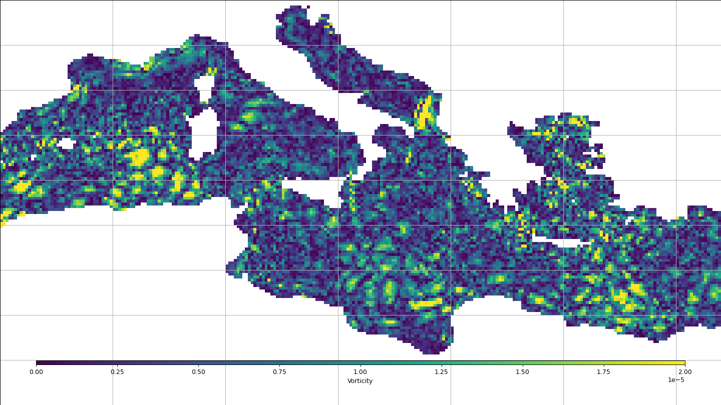
Display vorticity field

fig, ax, _ = start_ax()
mappable = g.display(ax, abs(g.grid("vort")), **kw_vorticity)
cb = update_axes(ax, mappable)
cb.set_label("Vorticity")

Particles

Particles specification

step = 1 / 32
x_g, y_g = arange(0, 36, step), arange(28, 46, step)
x, y = meshgrid(x_g, y_g)
original_shape = x.shape
x, y = x.reshape(-1), y.reshape(-1)
print(f"{len(x)} particles advected")
# A frame every 8h
step_by_day = 3
# Compute step of advection every 4h
nb_step = 2
kw_p = dict(
    nb_step=nb_step, time_step=86400 / step_by_day / nb_step, u_name="u", v_name="v"
)
# Start a generator which at each iteration return new position at next time step
particule = g.advect(x, y, **kw_p, rk4=True)

663552 particles advected

LAVD

lavd = zeros(original_shape)
# Advection time
nb_days = 8
# Nb frame
nb_time = step_by_day * nb_days
i = 0.0

Anim

Movie of LAVD integration at each integration time step.

def update(i_frame):
    global lavd, i
    i += 1
    x, y = particule.__next__()
    # Interp vorticity on new_position
    lavd += abs(g.interp("vort", x, y).reshape(original_shape) * 1 / nb_time)
    txt.set_text(f"T0 + {i / step_by_day:.2f} days of advection")
    pcolormesh.set_array(lavd / i * nb_time)
    return pcolormesh, txt


kw_video = dict(frames=arange(nb_time), interval=1000.0 / step_by_day / 2, blit=True)
fig, ax, txt = start_ax(dpi=60)
x_g_, y_g_ = (
    arange(0 - step / 2, 36 + step / 2, step),
    arange(28 - step / 2, 46 + step / 2, step),
)
# pcolorfast will be faster than pcolormesh, we could use pcolorfast due to x and y are regular
pcolormesh = ax.pcolorfast(x_g_, y_g_, lavd, **kw_vorticity)
update_axes(ax, pcolormesh)
_ = VideoAnimation(ax.figure, update, **kw_video)

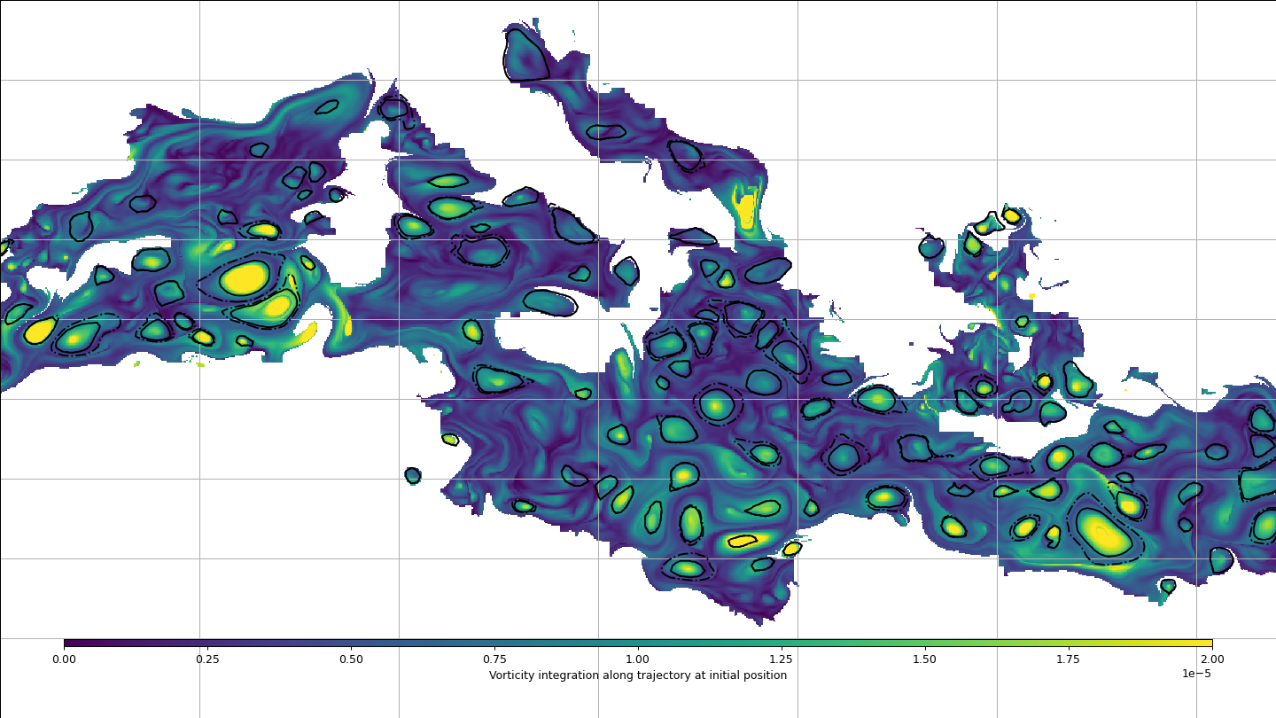
Final LAVD

Format LAVD data

lavd = RegularGridDataset.with_array(
    coordinates=("lon", "lat"), datas=dict(lavd=lavd.T, lon=x_g, lat=y_g), centered=True
)

Display final LAVD with py eddy tracker detection. Period used for LAVD integration (8 days) is too short for a real use, but choose for example efficiency.

fig, ax, _ = start_ax()
mappable = lavd.display(ax, "lavd", **kw_vorticity)
EddiesObservations.load_file(get_demo_path("Anticyclonic_20160515.nc")).display(
    ax, color="k"
)
EddiesObservations.load_file(get_demo_path("Cyclonic_20160515.nc")).display(
    ax, color="k"
)
_ = update_axes(ax, mappable)