Get Okubo Weis

\[OW = S_n^2 + S_s^2 + \omega^2\]

with normal strain (\(S_n\)), shear strain (\(S_s\)) and vorticity (\(\omega\))

\[S_n = \frac{\partial u}{\partial x} - \frac{\partial v}{\partial y}, S_s = \frac{\partial v}{\partial x} + \frac{\partial u}{\partial y}, \omega = \frac{\partial v}{\partial x} - \frac{\partial u}{\partial y}\]

from matplotlib import pyplot as plt
from numpy import arange, ma, where

from py_eddy_tracker import data
from py_eddy_tracker.dataset.grid import RegularGridDataset
from py_eddy_tracker.observations.observation import EddiesObservations

def start_axes(title, zoom=False):
    fig = plt.figure(figsize=(12, 6))
    axes = fig.add_axes([0.03, 0.03, 0.90, 0.94])
    axes.set_xlim(0, 360), axes.set_ylim(-80, 80)
    if zoom:
        axes.set_xlim(270, 340), axes.set_ylim(20, 50)
    axes.set_aspect("equal")
    axes.set_title(title)
    return axes


def update_axes(axes, mappable=None):
    axes.grid()
    if mappable:
        plt.colorbar(mappable, cax=axes.figure.add_axes([0.94, 0.05, 0.01, 0.9]))

Load detection files

a = EddiesObservations.load_file(data.get_demo_path("Anticyclonic_20190223.nc"))
c = EddiesObservations.load_file(data.get_demo_path("Cyclonic_20190223.nc"))

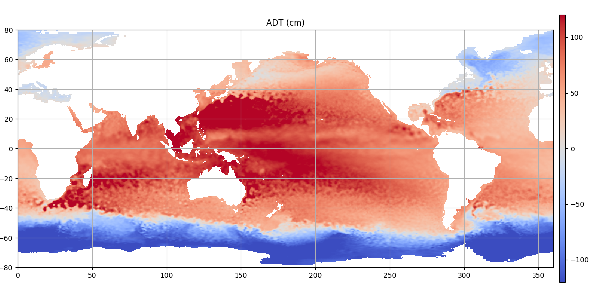
Load Input grid, ADT will be used to detect eddies

g = RegularGridDataset(
    data.get_demo_path("nrt_global_allsat_phy_l4_20190223_20190226.nc"),
    "longitude",
    "latitude",
)

ax = start_axes("ADT (cm)")
m = g.display(ax, "adt", vmin=-120, vmax=120, factor=100)
update_axes(ax, m)

Get parameter for ow

u_x = g.compute_stencil(g.grid("ugos"))
u_y = g.compute_stencil(g.grid("ugos"), vertical=True)
v_x = g.compute_stencil(g.grid("vgos"))
v_y = g.compute_stencil(g.grid("vgos"), vertical=True)
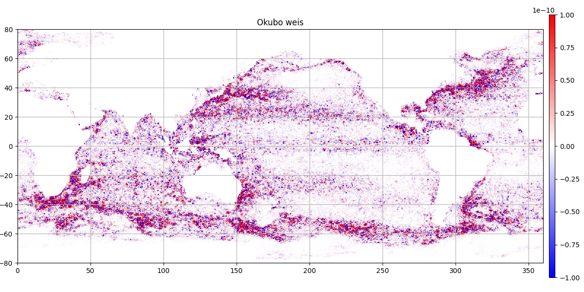
ow = g.vars["ow"] = (u_x - v_y) ** 2 + (v_x + u_y) ** 2 - (v_x - u_y) ** 2

ax = start_axes("Okubo weis")
m = g.display(ax, "ow", vmin=-1e-10, vmax=1e-10, cmap="bwr")
update_axes(ax, m)

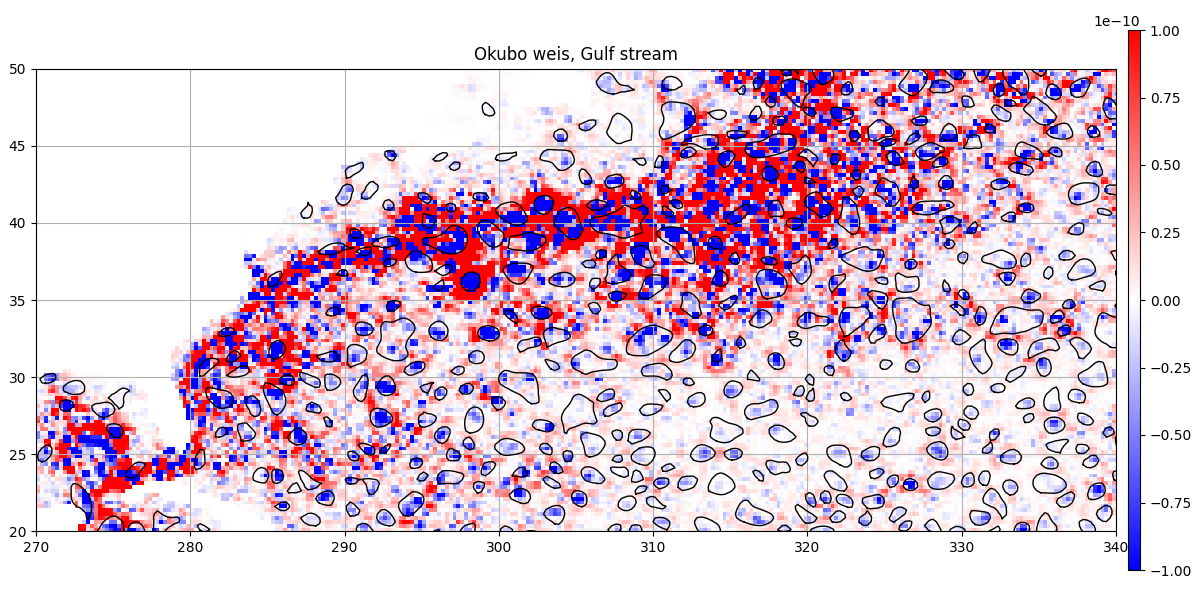
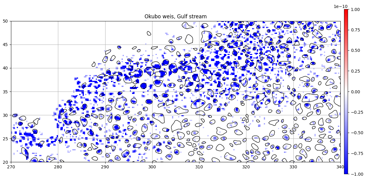
Gulf stream zoom

ax = start_axes("Okubo weis, Gulf stream", zoom=True)
m = g.display(ax, "ow", vmin=-1e-10, vmax=1e-10, cmap="bwr")
kw_ed = dict(intern_only=True, color="k", lw=1)
a.display(ax, **kw_ed), c.display(ax, **kw_ed)
update_axes(ax, m)

only negative OW

ax = start_axes("Okubo weis, Gulf stream", zoom=True)
threshold = ow.std() * -0.2
ow = ma.array(ow, mask=ow > threshold)
m = g.display(ax, ow, vmin=-1e-10, vmax=1e-10, cmap="bwr")
a.display(ax, **kw_ed), c.display(ax, **kw_ed)
update_axes(ax, m)

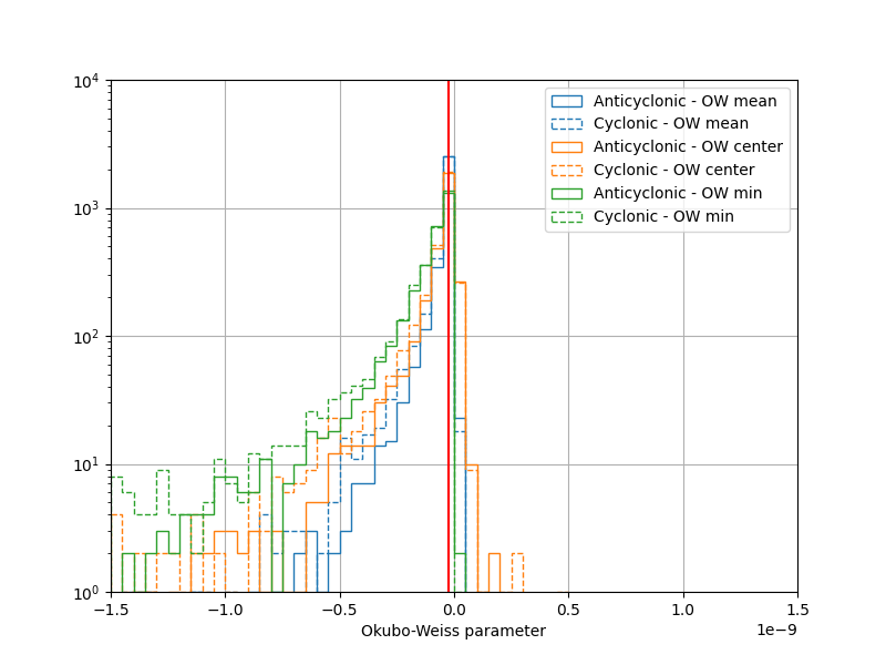
Get okubo-weiss mean/min/center in eddies

plt.figure(figsize=(8, 6))
ax = plt.subplot(111)
ax.set_xlabel("Okubo-Weiss parameter")
kw_hist = dict(bins=arange(-20e-10, 20e-10, 50e-12), histtype="step")
for method in ("mean", "center", "min"):
    kw_interp = dict(grid_object=g, varname="ow", method=method, intern=True)
    _, _, m = ax.hist(
        a.interp_grid(**kw_interp), label=f"Anticyclonic - OW {method}", **kw_hist
    )
    ax.hist(
        c.interp_grid(**kw_interp),
        label=f"Cyclonic - OW {method}",
        color=m[0].get_edgecolor(),
        ls="--",
        **kw_hist,
    )
ax.axvline(threshold, color="r")
ax.set_yscale("log")
ax.grid()
ax.set_ylim(1, 1e4)
ax.set_xlim(-15e-10, 15e-10)
ax.legend()

<matplotlib.legend.Legend object at 0x7f25162a78b0>

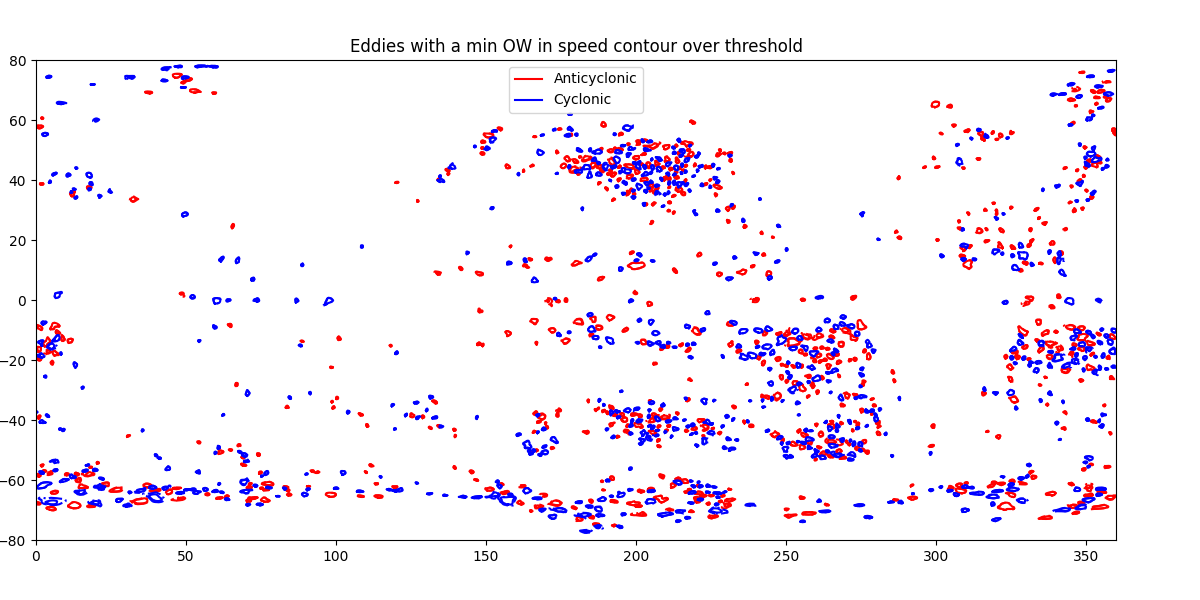
Catch eddies with bad OW

ax = start_axes("Eddies with a min OW in speed contour over threshold")
ow_min = a.interp_grid(**kw_interp)
a_bad_ow = a.index(where(ow_min > threshold)[0])
a_bad_ow.display(ax, color="r", label="Anticyclonic")
ow_min = c.interp_grid(**kw_interp)
c_bad_ow = c.index(where(ow_min > threshold)[0])
c_bad_ow.display(ax, color="b", label="Cyclonic")
ax.legend()

<matplotlib.legend.Legend object at 0x7f25195eb5e0>

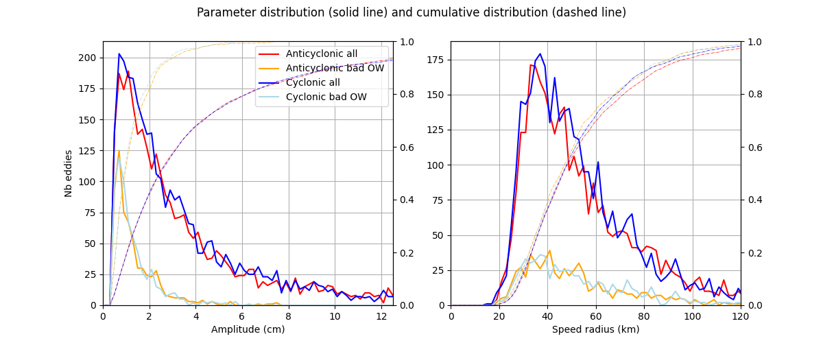
Display Radius and amplitude of eddies

fig = plt.figure(figsize=(12, 5))
fig.suptitle(
    "Parameter distribution (solid line) and cumulative distribution (dashed line)"
)
ax_amp, ax_rad = fig.add_subplot(121), fig.add_subplot(122)
ax_amp_c, ax_rad_c = ax_amp.twinx(), ax_rad.twinx()
ax_amp_c.set_ylim(0, 1), ax_rad_c.set_ylim(0, 1)
kw_a = dict(xname="amplitude", bins=arange(0, 2, 0.002).astype("f4"))
kw_r = dict(xname="radius_s", bins=arange(0, 500e6, 2e3).astype("f4"))
for d, label, color in (
    (a, "Anticyclonic all", "r"),
    (a_bad_ow, "Anticyclonic bad OW", "orange"),
    (c, "Cyclonic all", "blue"),
    (c_bad_ow, "Cyclonic bad OW", "lightblue"),
):
    x, y = d.bins_stat(**kw_a)
    ax_amp.plot(x * 100, y, label=label, color=color)
    ax_amp_c.plot(
        x * 100, y.cumsum() / y.sum(), label=label, color=color, ls="-.", lw=0.5
    )
    x, y = d.bins_stat(**kw_r)
    ax_rad.plot(x * 1e-3, y, label=label, color=color)
    ax_rad_c.plot(
        x * 1e-3, y.cumsum() / y.sum(), label=label, color=color, ls="-.", lw=0.5
    )

ax_amp.set_xlim(0, 12.5), ax_amp.grid(), ax_amp.set_ylim(0), ax_amp.legend()
ax_rad.set_xlim(0, 120), ax_rad.grid(), ax_rad.set_ylim(0)
ax_amp.set_xlabel("Amplitude (cm)"), ax_amp.set_ylabel("Nb eddies")
ax_rad.set_xlabel("Speed radius (km)")

Text(0.5, 25.722222222222214, 'Speed radius (km)')