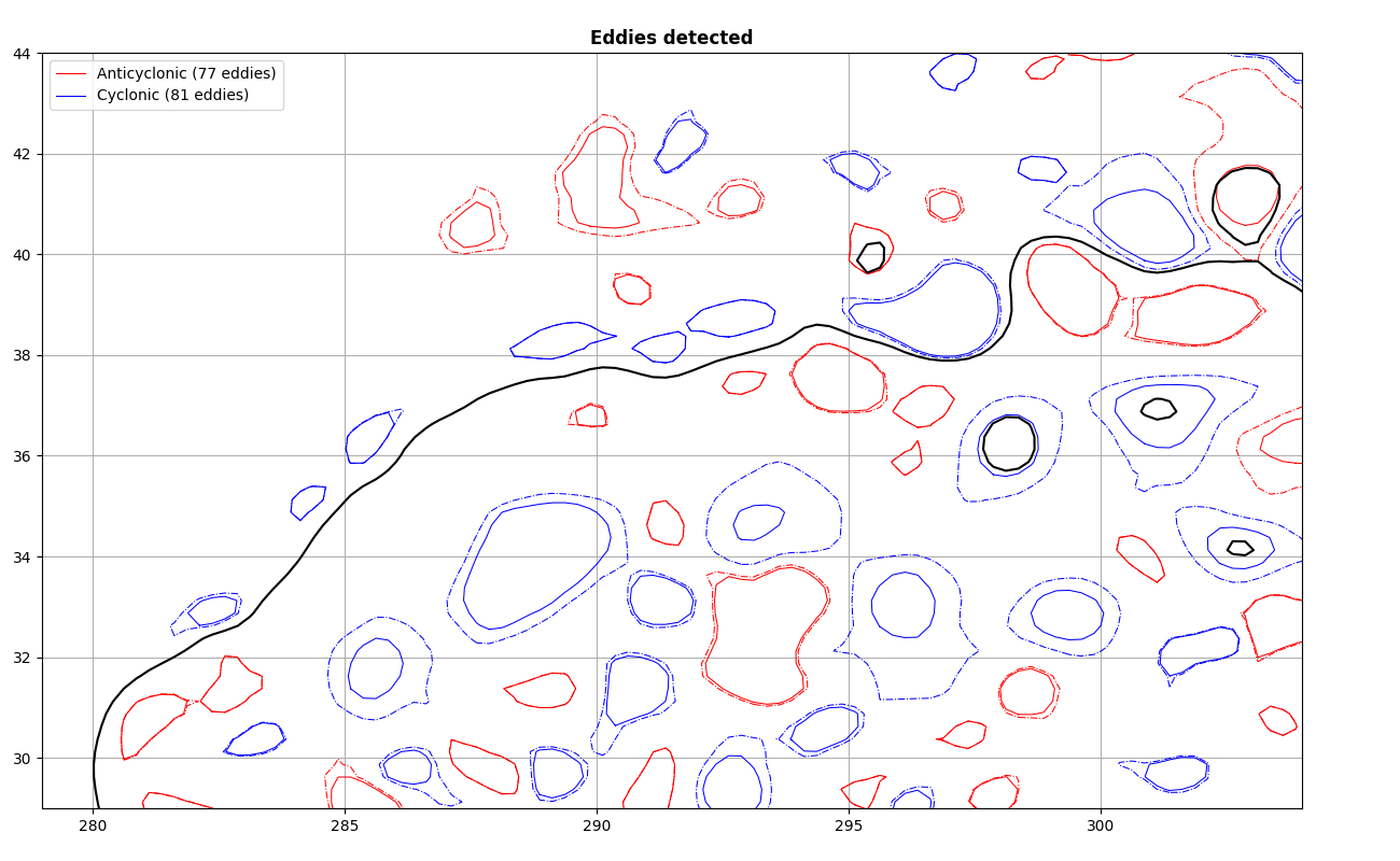
Eddy detection : Gulf stream

Script will detect eddies on adt field, and compute u,v with method add_uv(which could use, only if equator is avoid)

Figures will show different step to detect eddies.

from datetime import datetime

from matplotlib import pyplot as plt
from numpy import arange

from py_eddy_tracker import data
from py_eddy_tracker.dataset.grid import RegularGridDataset
from py_eddy_tracker.eddy_feature import Contours

def start_axes(title):
    fig = plt.figure(figsize=(13, 8))
    ax = fig.add_axes([0.03, 0.03, 0.90, 0.94])
    ax.set_xlim(279, 304), ax.set_ylim(29, 44)
    ax.set_aspect("equal")
    ax.set_title(title, weight="bold")
    return ax


def update_axes(ax, mappable=None):
    ax.grid()
    if mappable:
        plt.colorbar(mappable, cax=ax.figure.add_axes([0.94, 0.05, 0.01, 0.9]))

Load Input grid, ADT is used to detect eddies

margin = 30
g = RegularGridDataset(
    data.get_demo_path("nrt_global_allsat_phy_l4_20190223_20190226.nc"),
    "longitude",
    "latitude",
    # Manual area subset
    indexs=dict(
        longitude=slice(1116 - margin, 1216 + margin),
        latitude=slice(476 - margin, 536 + margin),
    ),
)

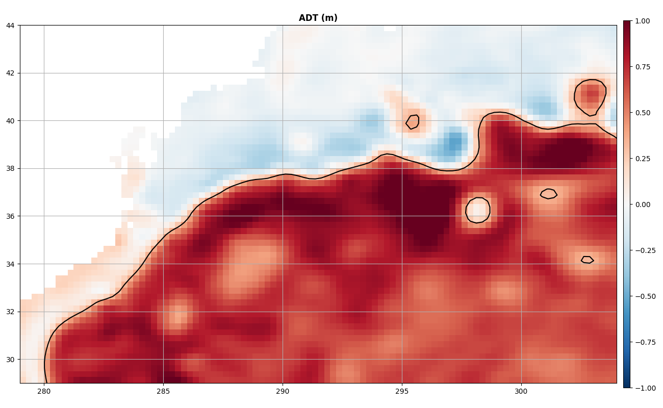
ax = start_axes("ADT (m)")
m = g.display(ax, "adt", vmin=-1, vmax=1, cmap="RdBu_r")
# Draw line on the gulf stream front
great_current = Contours(g.x_c, g.y_c, g.grid("adt"), levels=(0.35,), keep_unclose=True)
great_current.display(ax, color="k")
update_axes(ax, m)

Get geostrophic speed u,v

U/V are deduced from ADT, this algortihm is not ok near the equator (~+- 2°)

g.add_uv("adt")

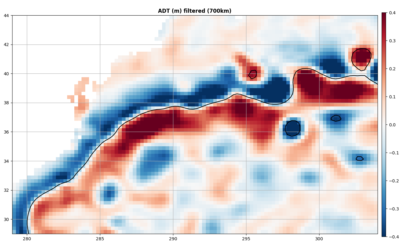
Pre-processings

Apply a high-pass filter to remove the large scale and highlight the mesoscale

g.bessel_high_filter("adt", 700)
ax = start_axes("ADT (m) filtered (700km)")
m = g.display(ax, "adt", vmin=-0.4, vmax=0.4, cmap="RdBu_r")
great_current.display(ax, color="k")
update_axes(ax, m)

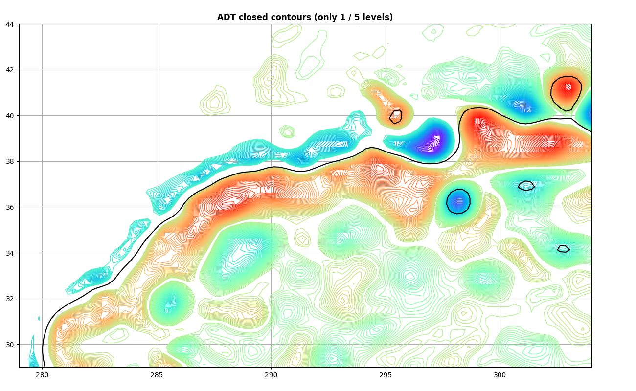
Identification

Run the identification step with slices of 2 mm

date = datetime(2016, 5, 15)
a, c = g.eddy_identification("adt", "u", "v", date, 0.002, shape_error=55)

/home/docs/checkouts/readthedocs.org/user_builds/py-eddy-tracker/conda/latest/lib/python3.10/site-packages/numpy-1.24.3-py3.10-linux-x86_64.egg/numpy/lib/function_base.py:4737: UserWarning: Warning: 'partition' will ignore the 'mask' of the MaskedArray.
  arr.partition(

Display of all closed contours found in the grid (only 1 contour every 5)

ax = start_axes("ADT closed contours (only 1 / 5 levels)")
g.contours.display(ax, step=5, lw=1)
great_current.display(ax, color="k")
update_axes(ax)

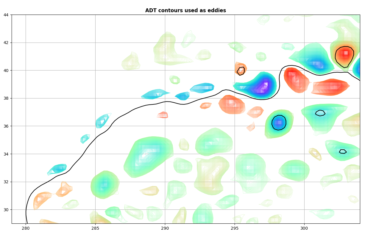
Contours included in eddies

ax = start_axes("ADT contours used as eddies")
g.contours.display(ax, only_used=True, lw=0.25)
great_current.display(ax, color="k")
update_axes(ax)

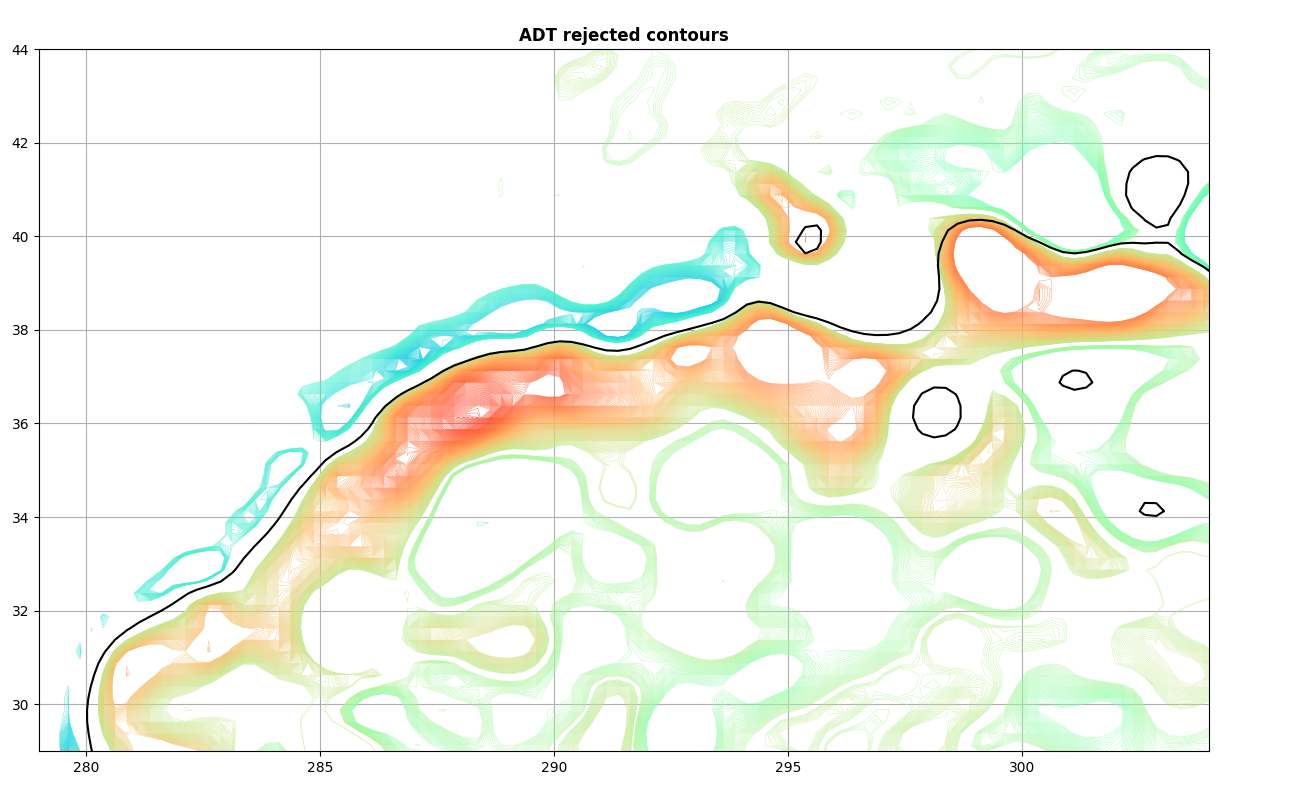
Post analysis

Contours can be rejected for several reasons (shape error to high, several extremum in contour, …)

ax = start_axes("ADT rejected contours")
g.contours.display(ax, only_unused=True, lw=0.25)
great_current.display(ax, color="k")
update_axes(ax)

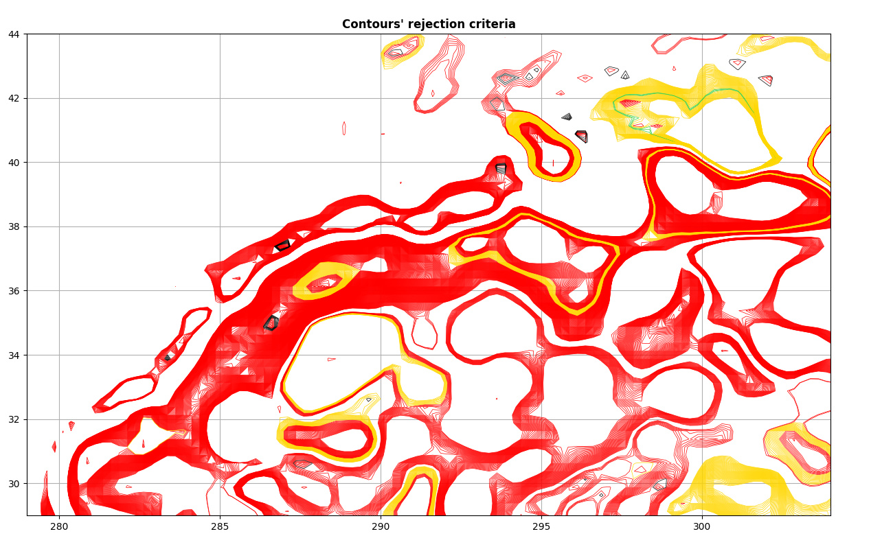
Criteria for rejecting a contour :

0. Accepted (green)

1. Rejection for shape error (red)

2. Masked value within contour (blue)

3. Under or over the pixel limit bounds (black)

4. Amplitude criterion (yellow)

ax = start_axes("Contours' rejection criteria")
g.contours.display(ax, only_unused=True, lw=0.5, display_criterion=True)
update_axes(ax)

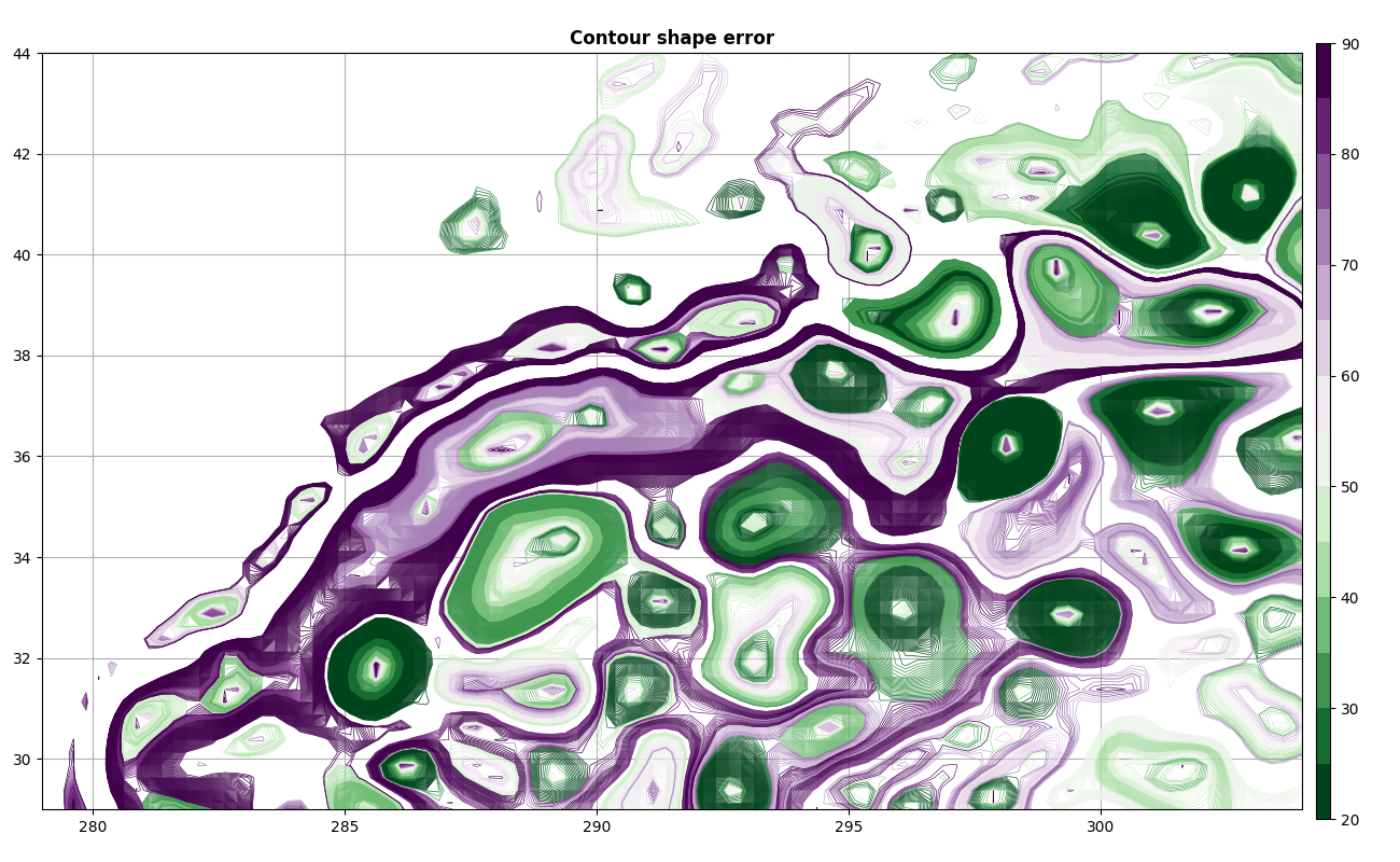
Display the shape error of each tested contour, the limit of shape error is set to 55 %

ax = start_axes("Contour shape error")
m = g.contours.display(
    ax, lw=0.5, field="shape_error", bins=arange(20, 90.1, 5), cmap="PRGn_r"
)
update_axes(ax, m)

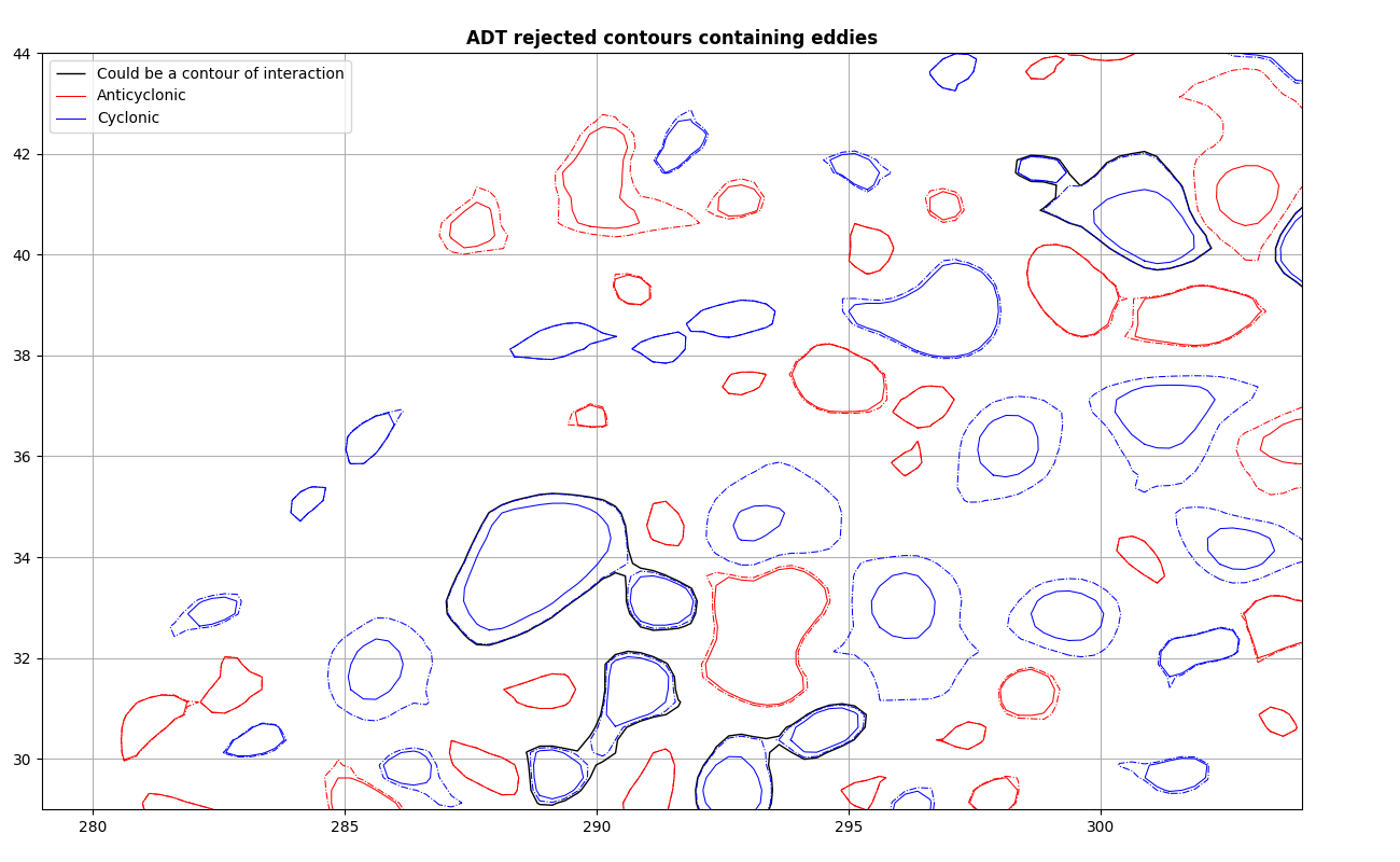
Some closed contours contains several eddies (aka, more than one extremum)

ax = start_axes("ADT rejected contours containing eddies")
g.contours.label_contour_unused_which_contain_eddies(a)
g.contours.label_contour_unused_which_contain_eddies(c)
g.contours.display(
    ax,
    only_contain_eddies=True,
    color="k",
    lw=1,
    label="Could be a contour of interaction",
)
a.display(ax, color="r", linewidth=0.75, label="Anticyclonic", ref=-10)
c.display(ax, color="b", linewidth=0.75, label="Cyclonic", ref=-10)
ax.legend()
update_axes(ax)

Output

When displaying the detected eddies, dashed lines are for effective contour, solide lines for the contour of the maximum mean speed. See figure 1 of https://doi.org/10.1175/JTECH-D-14-00019.1

ax = start_axes("Eddies detected")
a.display(
    ax, color="r", linewidth=0.75, label="Anticyclonic ({nb_obs} eddies)", ref=-10
)
c.display(ax, color="b", linewidth=0.75, label="Cyclonic ({nb_obs} eddies)", ref=-10)
ax.legend()
great_current.display(ax, color="k")
update_axes(ax)

Display the effective radius of the detected eddies

ax = start_axes("Effective radius (km)")
a.filled(ax, "radius_e", vmin=10, vmax=150, cmap="magma_r", factor=0.001, lut=14)
m = c.filled(ax, "radius_e", vmin=10, vmax=150, cmap="magma_r", factor=0.001, lut=14)
great_current.display(ax, color="k")
update_axes(ax, m)