Display identification

from matplotlib import pyplot as plt

from py_eddy_tracker import data
from py_eddy_tracker.observations.observation import EddiesObservations

Load detection files

a = EddiesObservations.load_file(data.get_demo_path("Anticyclonic_20190223.nc"))
c = EddiesObservations.load_file(data.get_demo_path("Cyclonic_20190223.nc"))

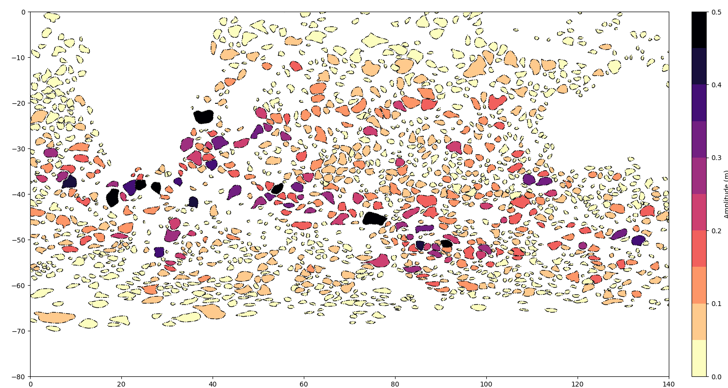
Fill effective contour with amplitude

fig = plt.figure(figsize=(15, 8))
ax = fig.add_axes([0.03, 0.03, 0.90, 0.94])
ax.set_aspect("equal")
ax.set_xlim(0, 140)
ax.set_ylim(-80, 0)
kwargs = dict(extern_only=True, color="k", lw=1)
a.display(ax, **kwargs), c.display(ax, **kwargs)
a.filled(ax, "amplitude", cmap="magma_r", vmin=0, vmax=0.5)
m = c.filled(ax, "amplitude", cmap="magma_r", vmin=0, vmax=0.5)
colorbar = plt.colorbar(m, cax=ax.figure.add_axes([0.95, 0.03, 0.02, 0.94]))
colorbar.set_label("Amplitude (m)")

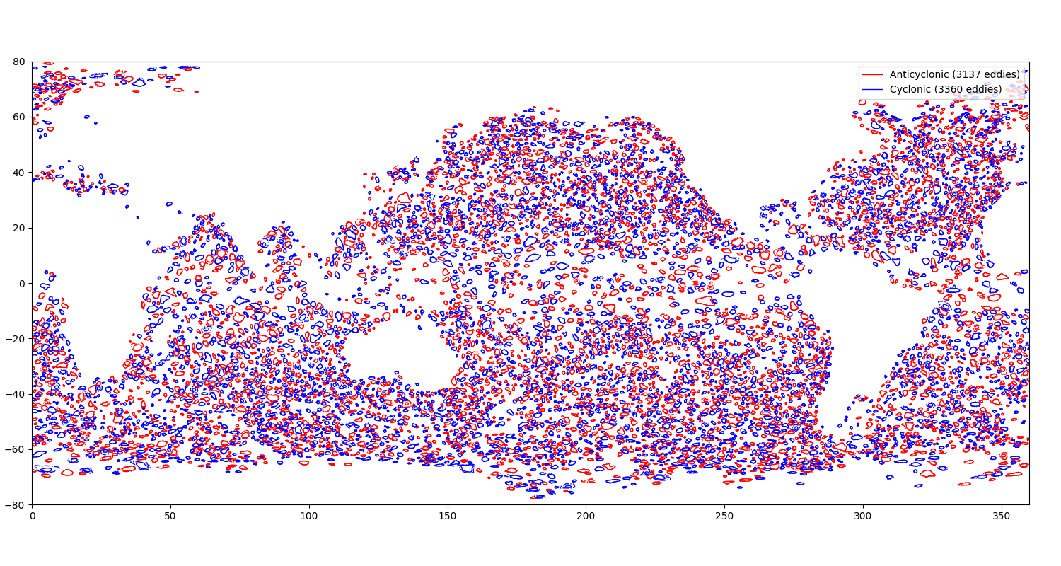
Draw speed contours

fig = plt.figure(figsize=(15, 8))
ax = fig.add_axes([0.03, 0.03, 0.94, 0.94])
ax.set_aspect("equal")
ax.set_xlim(0, 360)
ax.set_ylim(-80, 80)
a.display(ax, label="Anticyclonic ({nb_obs} eddies)", color="r", lw=1)
c.display(ax, label="Cyclonic ({nb_obs} eddies)", color="b", lw=1)
ax.legend(loc="upper right")

<matplotlib.legend.Legend object at 0x749040d0a630>

Get general informations

print(a)

| 3137 observations from 25255.0 to 25255.0 (1.0 days, ~3137 obs/day)
|   Speed area      : 32.98 Mkm²/day
|   Effective area  : 45.65 Mkm²/day
----Distribution in Amplitude:
|   Amplitude bounds (cm)        0.00      1.00      2.00      3.00      4.00      5.00     10.00    500.00
|   Percent of eddies         :      19.35     22.73     15.40     10.30      6.18     15.91     10.14
----Distribution in Radius:
|   Speed radius (km)            0.00     15.00     30.00     45.00     60.00     75.00    100.00    200.00   2000.00
|   Percent of eddies         :       0.00      9.47     34.56     24.55     13.29     11.67      6.34      0.13
|   Effective radius (km)        0.00     15.00     30.00     45.00     60.00     75.00    100.00    200.00   2000.00
|   Percent of eddies         :       0.00      7.52     26.62     20.88     15.40     15.94     13.32      0.32
----Distribution in Latitude
    Latitude bounds            -90.00    -60.00    -15.00     15.00     60.00     90.00
    Percent of eddies         :       7.62     46.86     12.81     30.06      2.65
    Percent of speed area     :       4.69     41.94     26.90     25.30      1.17
    Percent of effective area :       4.74     43.40     25.53     25.11      1.21
    Mean speed radius (km)    :      43.94     52.75     81.69     51.01     37.91
    Mean effective radius (km):      52.14     62.43     94.14     59.44     44.81
    Mean amplitude (cm)       :       3.53      5.30      2.19      4.32      3.12

print(c)

| 3360 observations from 25255.0 to 25255.0 (1.0 days, ~3360 obs/day)
|   Speed area      : 32.89 Mkm²/day
|   Effective area  : 46.42 Mkm²/day
----Distribution in Amplitude:
|   Amplitude bounds (cm)        0.00      1.00      2.00      3.00      4.00      5.00     10.00    500.00
|   Percent of eddies         :      18.81     24.02     14.11     10.89      5.98     16.19     10.00
----Distribution in Radius:
|   Speed radius (km)            0.00     15.00     30.00     45.00     60.00     75.00    100.00    200.00   2000.00
|   Percent of eddies         :       0.03     10.15     35.03     25.15     14.40     10.09      5.12      0.03
|   Effective radius (km)        0.00     15.00     30.00     45.00     60.00     75.00    100.00    200.00   2000.00
|   Percent of eddies         :       0.03      7.98     26.88     21.61     15.92     15.09     12.14      0.36
----Distribution in Latitude
    Latitude bounds            -90.00    -60.00    -15.00     15.00     60.00     90.00
    Percent of eddies         :       7.92     46.96     13.12     29.61      2.38
    Percent of speed area     :       4.80     41.08     27.30     25.87      0.93
    Percent of effective area :       4.83     42.35     25.36     26.55      0.92
    Mean speed radius (km)    :      42.23     50.71     78.76     50.80     34.64
    Mean effective radius (km):      49.25     60.50     89.91     59.96     40.20
    Mean amplitude (cm)       :       3.19      5.71      2.19      4.24      2.42