Stastics on identification files

Some statistics on raw identification without any tracking

from matplotlib import pyplot as plt
from matplotlib.dates import date2num
import numpy as np

from py_eddy_tracker import start_logger
from py_eddy_tracker.data import get_remote_demo_sample
from py_eddy_tracker.observations.observation import EddiesObservations

start_logger().setLevel("ERROR")

def start_axes(title):
    fig = plt.figure(figsize=(13, 5))
    ax = fig.add_axes([0.03, 0.03, 0.90, 0.94])
    ax.set_xlim(-6, 36.5), ax.set_ylim(30, 46)
    ax.set_aspect("equal")
    ax.set_title(title)
    return ax


def update_axes(ax, mappable=None):
    ax.grid()
    if mappable:
        plt.colorbar(mappable, cax=ax.figure.add_axes([0.95, 0.05, 0.01, 0.9]))

We load demo sample and take only first year.

Replace by a list of filename to apply on your own dataset.

file_objects = get_remote_demo_sample(
    "eddies_med_adt_allsat_dt2018/Anticyclonic_2010_2011_2012"
)[:365]

Merge all identification datasets in one object

all_a = EddiesObservations.concatenate(
    [EddiesObservations.load_file(i) for i in file_objects]
)

We define polygon bound

x0, x1, y0, y1 = 15, 20, 33, 38
xs = np.array([[x0, x1, x1, x0, x0]], dtype="f8")
ys = np.array([[y0, y0, y1, y1, y0]], dtype="f8")
# Polygon object created for the match function use.
polygon = dict(contour_lon_e=xs, contour_lat_e=ys, contour_lon_s=xs, contour_lat_s=ys)

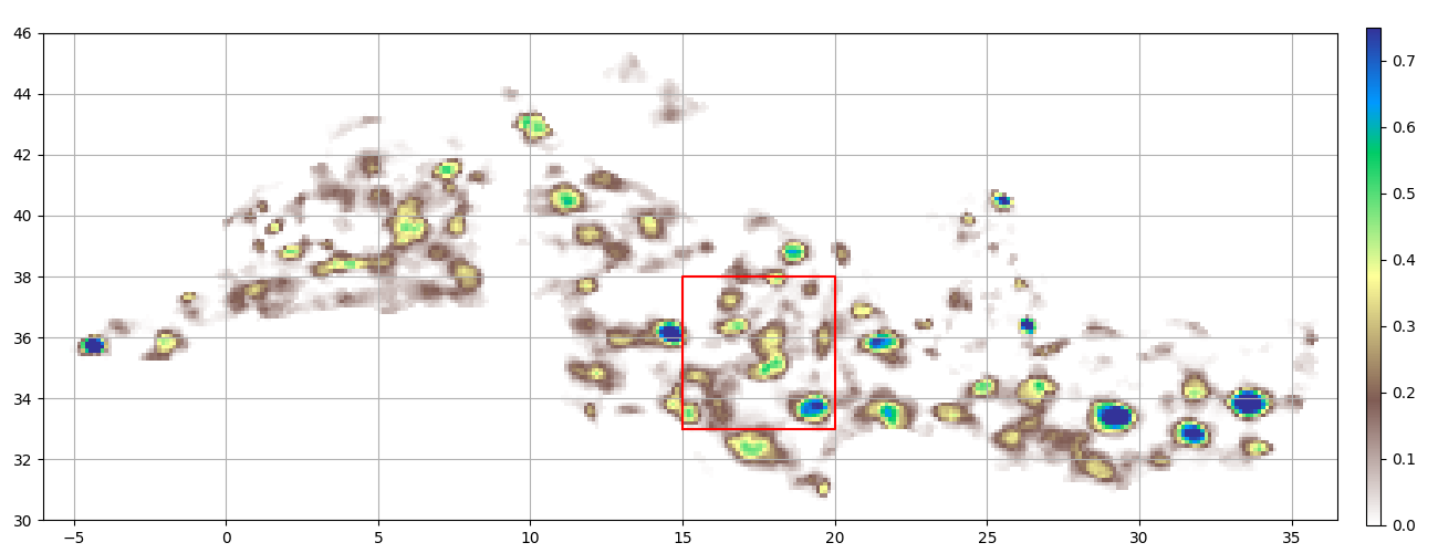
Geographic frequency of eddies

step = 0.125
ax = start_axes("")
# Count pixel encompassed in each contour
g_a = all_a.grid_count(bins=((-10, 37, step), (30, 46, step)), intern=True)
m = g_a.display(
    ax, cmap="terrain_r", vmin=0, vmax=0.75, factor=1 / all_a.nb_days, name="count"
)
ax.plot(polygon["contour_lon_e"][0], polygon["contour_lat_e"][0], "r")
update_axes(ax, m)

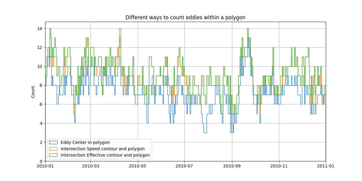
We use the match function to count the number of eddies that intersect the polygon defined previously p1_area option allow to get in c_e/c_s output, precentage of area occupy by eddies in the polygon.

i_e, j_e, c_e = all_a.match(polygon, p1_area=True, intern=False)
i_s, j_s, c_s = all_a.match(polygon, p1_area=True, intern=True)

dt = np.datetime64("1970-01-01") - np.datetime64("1950-01-01")
kw_hist = dict(
    bins=date2num(np.arange(21900, 22300).astype("datetime64") - dt), histtype="step"
)
# translate julian day in datetime64
t = all_a.time.astype("datetime64") - dt

Number of eddies within a polygon

ax = plt.figure(figsize=(12, 6)).add_subplot(111)
ax.set_title("Different ways to count eddies within a polygon")
ax.set_ylabel("Count")
m = all_a.mask_from_polygons(((xs, ys),))
ax.hist(t[m], label="Eddy Center in polygon", **kw_hist)
ax.hist(t[i_s[c_s > 0]], label="Intersection Speed contour and polygon", **kw_hist)
ax.hist(t[i_e[c_e > 0]], label="Intersection Effective contour and polygon", **kw_hist)
ax.legend()
ax.set_xlim(np.datetime64("2010"), np.datetime64("2011"))
ax.grid()

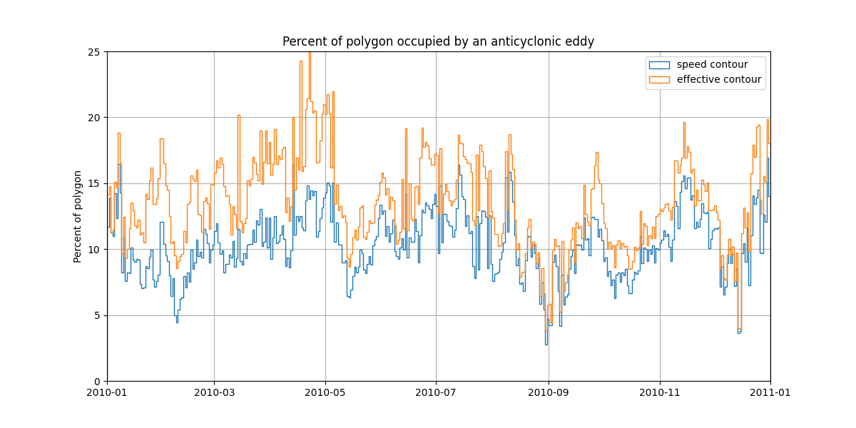
Percent of the area of interest occupied by eddies.

ax = plt.figure(figsize=(12, 6)).add_subplot(111)
ax.set_title("Percent of polygon occupied by an anticyclonic eddy")
ax.set_ylabel("Percent of polygon")
ax.hist(t[i_s[c_s > 0]], weights=c_s[c_s > 0] * 100.0, label="speed contour", **kw_hist)
ax.hist(
    t[i_e[c_e > 0]], weights=c_e[c_e > 0] * 100.0, label="effective contour", **kw_hist
)
ax.legend(), ax.set_ylim(0, 25)
ax.set_xlim(np.datetime64("2010"), np.datetime64("2011"))
ax.grid()