Eddy detection : Antartic Circumpolar Current

This script detect eddies on the ADT field, and compute u,v with the method add_uv (use it only if the Equator is avoided)

Two detections are provided : with a filtered ADT and without filtering

from datetime import datetime

from matplotlib import pyplot as plt, style

from py_eddy_tracker import data
from py_eddy_tracker.dataset.grid import RegularGridDataset

pos_cb = [0.1, 0.52, 0.83, 0.015]
pos_cb2 = [0.1, 0.07, 0.4, 0.015]


def quad_axes(title):
    style.use("default")
    fig = plt.figure(figsize=(13, 10))
    fig.suptitle(title, weight="bold", fontsize=14)
    axes = list()

    ax_pos = dict(
        topleft=[0.1, 0.54, 0.4, 0.38],
        topright=[0.53, 0.54, 0.4, 0.38],
        botleft=[0.1, 0.09, 0.4, 0.38],
        botright=[0.53, 0.09, 0.4, 0.38],
    )

    for key, position in ax_pos.items():
        ax = fig.add_axes(position)
        ax.set_xlim(5, 45), ax.set_ylim(-60, -37)
        ax.set_aspect("equal"), ax.grid(True)
        axes.append(ax)
        if "right" in key:
            ax.set_yticklabels("")
    return fig, axes


def set_fancy_labels(fig, ticklabelsize=14, labelsize=14, labelweight="semibold"):
    for ax in fig.get_axes():
        ax.grid()
        ax.grid(which="major", linestyle="-", linewidth="0.5", color="black")
        if ax.get_ylabel() != "":
            ax.set_ylabel(ax.get_ylabel(), fontsize=labelsize, fontweight=labelweight)
        if ax.get_xlabel() != "":
            ax.set_xlabel(ax.get_xlabel(), fontsize=labelsize, fontweight=labelweight)
        if ax.get_title() != "":
            ax.set_title(ax.get_title(), fontsize=labelsize, fontweight=labelweight)
        ax.tick_params(labelsize=ticklabelsize)

Load Input grid, ADT is used to detect eddies

margin = 30

kw_data = dict(
    filename=data.get_demo_path("nrt_global_allsat_phy_l4_20190223_20190226.nc"),
    x_name="longitude",
    y_name="latitude",
    # Manual area subset
    indexs=dict(
        latitude=slice(100 - margin, 220 + margin),
        longitude=slice(0, 230 + margin),
    ),
)
g_raw = RegularGridDataset(**kw_data)
g_raw.add_uv("adt")
g = RegularGridDataset(**kw_data)
g.copy("adt", "adt_low")
g.bessel_high_filter("adt", 700)
g.bessel_low_filter("adt_low", 700)
g.add_uv("adt")

Identification

Run the identification step with slices of 2 mm

date = datetime(2016, 5, 15)
kw_ident = dict(
    date=date, step=0.002, shape_error=70, sampling=30, uname="u", vname="v"
)
a, c = g.eddy_identification("adt", **kw_ident)
a_, c_ = g_raw.eddy_identification("adt", **kw_ident)

/home/docs/checkouts/readthedocs.org/user_builds/py-eddy-tracker/conda/latest/lib/python3.10/site-packages/numpy-1.24.3-py3.10-linux-x86_64.egg/numpy/lib/function_base.py:4737: UserWarning: Warning: 'partition' will ignore the 'mask' of the MaskedArray.
  arr.partition(

Figures

kw_adt = dict(vmin=-1.5, vmax=1.5, cmap=plt.get_cmap("RdBu_r", 30))
fig, axs = quad_axes("General properties field")
g_raw.display(axs[0], "adt", **kw_adt)
axs[0].set_title("Total ADT (m)")
m = g.display(axs[1], "adt_low", **kw_adt)
axs[1].set_title("ADT (m) large scale, cutoff at 700 km")
m2 = g.display(axs[2], "adt", cmap=plt.get_cmap("RdBu_r", 20), vmin=-0.5, vmax=0.5)
axs[2].set_title("ADT (m) high-pass filtered, a cutoff at 700 km")
cb = plt.colorbar(m, cax=axs[0].figure.add_axes(pos_cb), orientation="horizontal")
cb.set_label("ADT (m)", labelpad=0)
cb2 = plt.colorbar(m2, cax=axs[2].figure.add_axes(pos_cb2), orientation="horizontal")
cb2.set_label("ADT (m)", labelpad=0)
set_fancy_labels(fig)

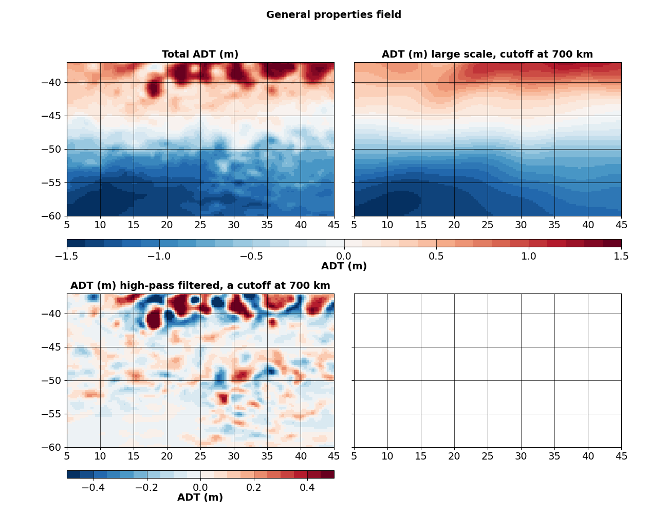
The large-scale North-South gradient is removed by the filtering step.

fig, axs = quad_axes("")
axs[0].set_title("Without filter")
axs[0].set_ylabel("Contours used in eddies")
axs[1].set_title("With filter")
axs[2].set_ylabel("Closed contours but not used")
g_raw.contours.display(axs[0], lw=0.5, only_used=True)
g.contours.display(axs[1], lw=0.5, only_used=True)
g_raw.contours.display(axs[2], lw=0.5, only_unused=True)
g.contours.display(axs[3], lw=0.5, only_unused=True)
set_fancy_labels(fig)

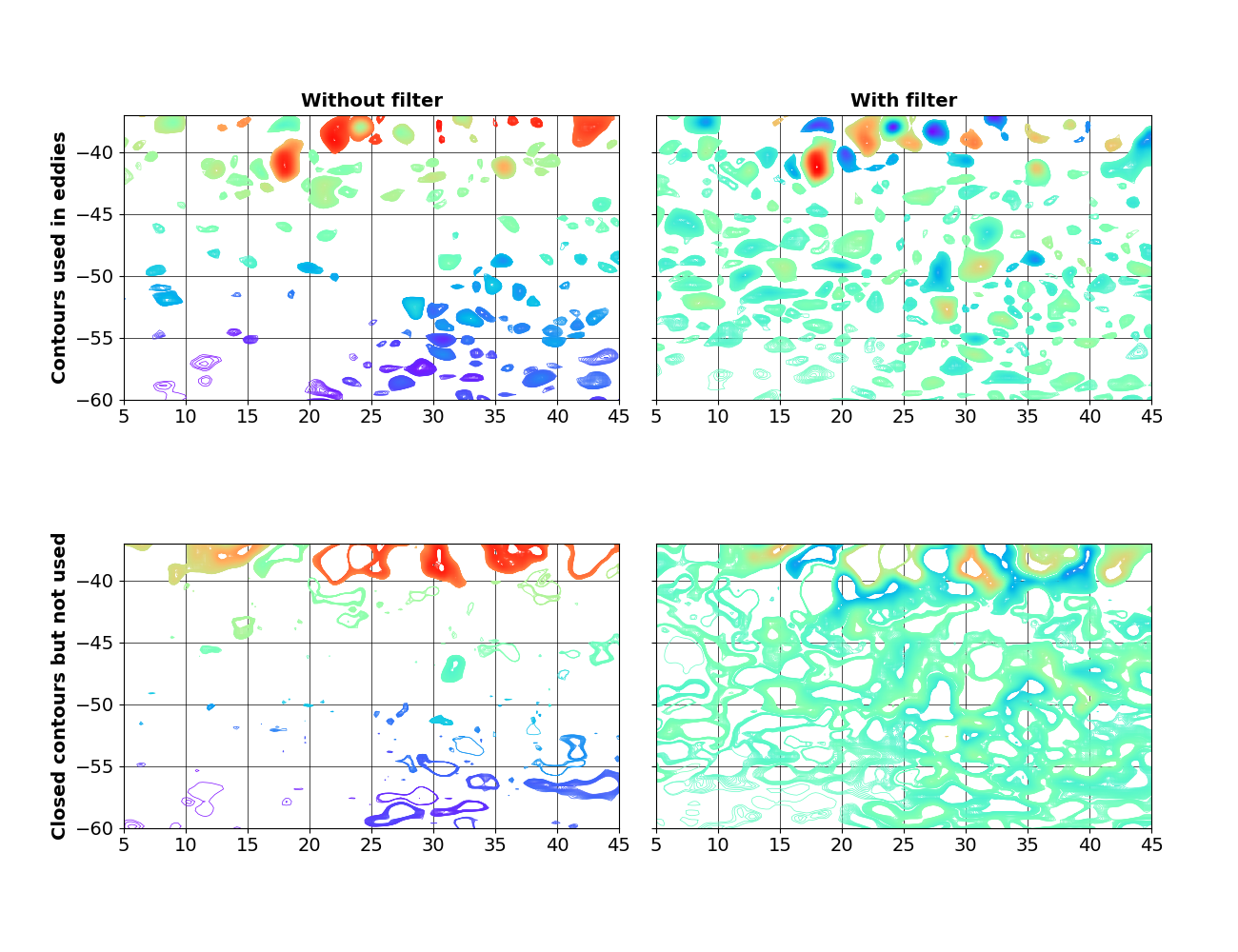
Removing the large-scale North-South gradient reveals closed contours in the South-Western corner of the ewample region.

kw = dict(ref=-10, linewidth=0.75)
kw_a = dict(color="r", label="Anticyclonic ({nb_obs} eddies)")
kw_c = dict(color="b", label="Cyclonic ({nb_obs} eddies)")
kw_filled = dict(vmin=0, vmax=100, cmap="Spectral_r", lut=20, intern=True, factor=100)
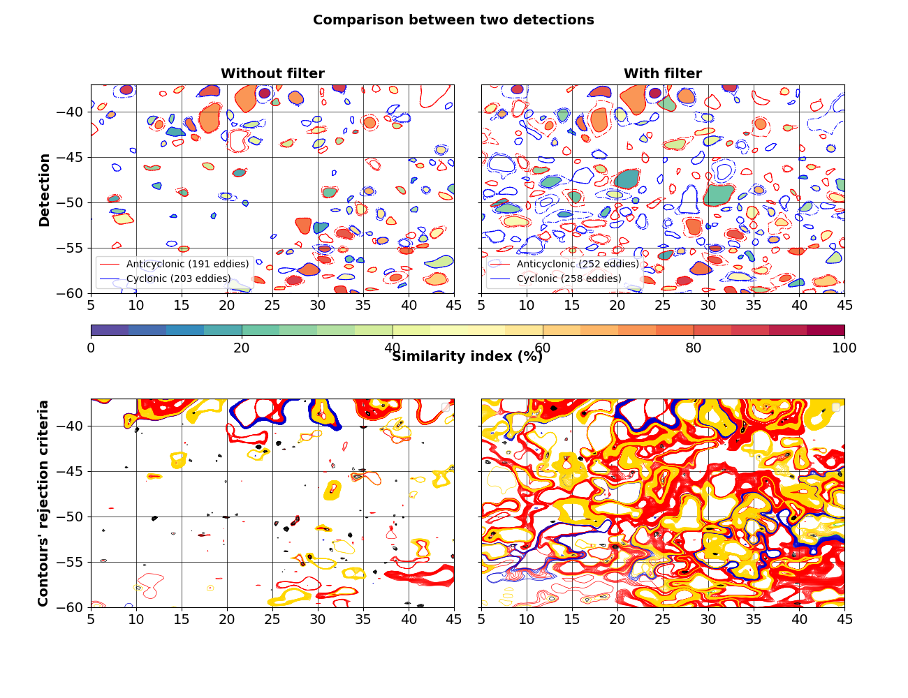
fig, axs = quad_axes("Comparison between two detections")
# Match with intern/inner contour
i_a, j_a, s_a = a_.match(a, intern=True, cmin=0.15)
i_c, j_c, s_c = c_.match(c, intern=True, cmin=0.15)

a_.index(i_a).filled(axs[0], s_a, **kw_filled)
a.index(j_a).filled(axs[1], s_a, **kw_filled)
c_.index(i_c).filled(axs[0], s_c, **kw_filled)
m = c.index(j_c).filled(axs[1], s_c, **kw_filled)

cb = plt.colorbar(m, cax=axs[0].figure.add_axes(pos_cb), orientation="horizontal")
cb.set_label("Similarity index (%)", labelpad=-5)
a_.display(axs[0], **kw, **kw_a), c_.display(axs[0], **kw, **kw_c)
a.display(axs[1], **kw, **kw_a), c.display(axs[1], **kw, **kw_c)

axs[0].set_title("Without filter")
axs[0].set_ylabel("Detection")
axs[1].set_title("With filter")
axs[2].set_ylabel("Contours' rejection criteria")

g_raw.contours.display(axs[2], lw=0.5, only_unused=True, display_criterion=True)
g.contours.display(axs[3], lw=0.5, only_unused=True, display_criterion=True)

for ax in axs:
    ax.legend()

set_fancy_labels(fig)

No artists with labels found to put in legend.  Note that artists whose label start with an underscore are ignored when legend() is called with no argument.
No artists with labels found to put in legend.  Note that artists whose label start with an underscore are ignored when legend() is called with no argument.

Very similar eddies have Similarity Indexes >= 40%

Criteria for rejecting a contour :

0. Accepted (green)

1. Rejection for shape error (red)

2. Masked value within contour (blue)

3. Under or over the pixel limit bounds (black)

4. Amplitude criterion (yellow)

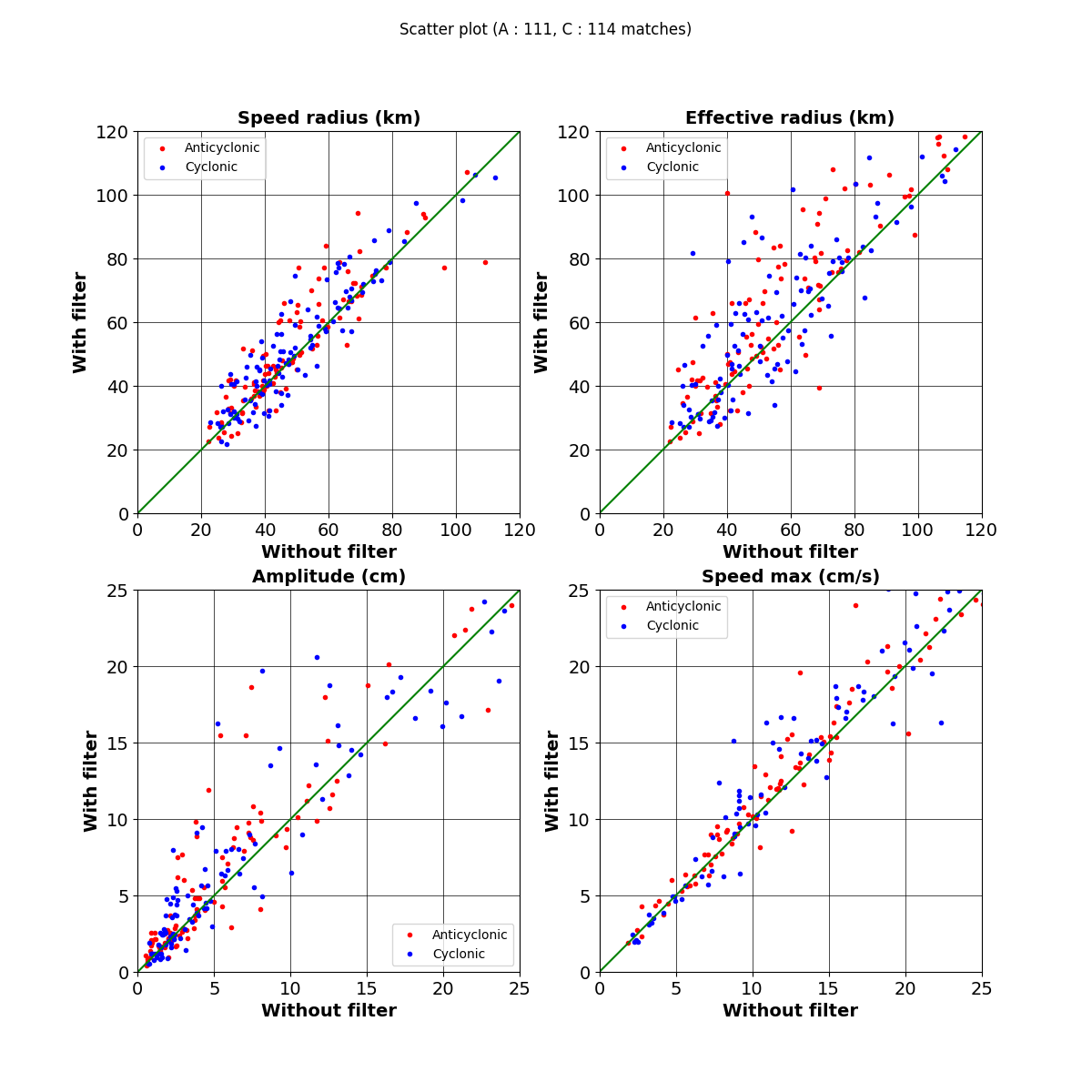
i_a, j_a = i_a[s_a >= 0.4], j_a[s_a >= 0.4]
i_c, j_c = i_c[s_c >= 0.4], j_c[s_c >= 0.4]
fig = plt.figure(figsize=(12, 12))
fig.suptitle(f"Scatter plot (A : {i_a.shape[0]}, C : {i_c.shape[0]} matches)")

for i, (label, field, factor, stop) in enumerate(
    (
        ("Speed radius (km)", "radius_s", 0.001, 120),
        ("Effective radius (km)", "radius_e", 0.001, 120),
        ("Amplitude (cm)", "amplitude", 100, 25),
        ("Speed max (cm/s)", "speed_average", 100, 25),
    )
):
    ax = fig.add_subplot(2, 2, i + 1, title=label)
    ax.set_xlabel("Without filter")
    ax.set_ylabel("With filter")

    ax.plot(
        a_[field][i_a] * factor,
        a[field][j_a] * factor,
        "r.",
        label="Anticyclonic",
    )
    ax.plot(
        c_[field][i_c] * factor,
        c[field][j_c] * factor,
        "b.",
        label="Cyclonic",
    )
    ax.set_aspect("equal"), ax.grid()
    ax.plot((0, 1000), (0, 1000), "g")
    ax.set_xlim(0, stop), ax.set_ylim(0, stop)
    ax.legend()

set_fancy_labels(fig)