Collocating external data

Script will use py-eddy-tracker methods to upload external data (sea surface temperature, SST) in a common structure with altimetry.

Figures higlights the different steps.

from datetime import datetime

from matplotlib import pyplot as plt

from py_eddy_tracker import data
from py_eddy_tracker.dataset.grid import RegularGridDataset

date = datetime(2016, 7, 7)

filename_alt = data.get_demo_path(
    f"dt_blacksea_allsat_phy_l4_{date:%Y%m%d}_20200801.nc"
)
filename_sst = data.get_demo_path(
    f"{date:%Y%m%d}000000-GOS-L4_GHRSST-SSTfnd-OISST_HR_REP-BLK-v02.0-fv01.0.nc"
)
var_name_sst = "analysed_sst"

extent = [27, 42, 40.5, 47]

Loading data

sst = RegularGridDataset(filename=filename_sst, x_name="lon", y_name="lat")
alti = RegularGridDataset(
    data.get_demo_path(filename_alt), x_name="longitude", y_name="latitude"
)
# We can use `Grid` tools to interpolate ADT on the sst grid
sst.regrid(alti, "sla")
sst.add_uv("sla")

Functions to initiate figure axes

def start_axes(title, extent=extent):
    fig = plt.figure(figsize=(13, 6), dpi=120)
    ax = fig.add_axes([0.03, 0.05, 0.89, 0.91])
    ax.set_xlim(extent[0], extent[1])
    ax.set_ylim(extent[2], extent[3])
    ax.set_title(title)
    ax.set_aspect("equal")
    return ax


def update_axes(ax, mappable=None, unit=""):
    ax.grid()
    if mappable:
        cax = ax.figure.add_axes([0.93, 0.05, 0.01, 0.9], title=unit)
        plt.colorbar(mappable, cax=cax)

ADT first display

ax = start_axes("SLA", extent=extent)
m = sst.display(ax, "sla", vmin=0.05, vmax=0.35)
update_axes(ax, m, unit="[m]")

SST first display

We can now plot SST from sst

ax = start_axes("SST")
m = sst.display(ax, "analysed_sst", vmin=295, vmax=300)
update_axes(ax, m, unit="[°K]")

ax = start_axes("SST")
m = sst.display(ax, "analysed_sst", vmin=295, vmax=300)
u, v = sst.grid("u").T, sst.grid("v").T
ax.quiver(sst.x_c[::3], sst.y_c[::3], u[::3, ::3], v[::3, ::3], scale=10)
update_axes(ax, m, unit="[°K]")

Now, with eddy contours, and displaying SST anomaly

sst.bessel_high_filter("analysed_sst", 400)

Eddy detection

sst.bessel_high_filter("sla", 400)
# ADT filtered
ax = start_axes("SLA", extent=extent)
m = sst.display(ax, "sla", vmin=-0.1, vmax=0.1)
update_axes(ax, m, unit="[m]")
a, c = sst.eddy_identification("sla", "u", "v", date, 0.002)

/home/docs/checkouts/readthedocs.org/user_builds/py-eddy-tracker/conda/latest/lib/python3.10/site-packages/numpy-1.24.3-py3.10-linux-x86_64.egg/numpy/lib/function_base.py:4737: UserWarning: Warning: 'partition' will ignore the 'mask' of the MaskedArray.
  arr.partition(

kwargs_a = dict(lw=2, label="Anticyclonic", ref=-10, color="b")
kwargs_c = dict(lw=2, label="Cyclonic", ref=-10, color="r")
ax = start_axes("SST anomaly")
m = sst.display(ax, "analysed_sst", vmin=-1, vmax=1)
a.display(ax, **kwargs_a), c.display(ax, **kwargs_c)
ax.legend()
update_axes(ax, m, unit="[°K]")

Example of post-processing

Get mean of sst anomaly_high in each internal contour

anom_a = a.interp_grid(sst, "analysed_sst", method="mean", intern=True)
anom_c = c.interp_grid(sst, "analysed_sst", method="mean", intern=True)

Are cyclonic (resp. anticyclonic) eddies generally associated with positive (resp. negative) SST anomaly ?

fig = plt.figure(figsize=(7, 5))
ax = fig.add_axes([0.05, 0.05, 0.90, 0.90])
ax.set_xlabel("SST anomaly")
ax.set_xlim([-1, 1])
ax.set_title("Histograms of SST anomalies")
ax.hist(
    anom_a, 5, alpha=0.5, color="b", label="Anticyclonic (mean:%s)" % (anom_a.mean())
)
ax.hist(anom_c, 5, alpha=0.5, color="r", label="Cyclonic (mean:%s)" % (anom_c.mean()))
ax.legend()

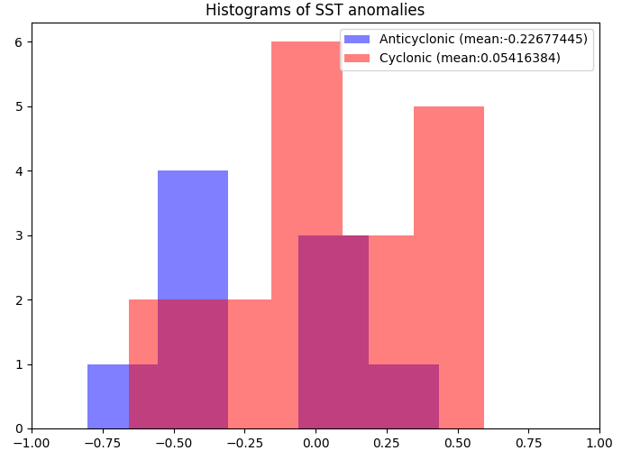
<matplotlib.legend.Legend object at 0x7f2516583100>

Not clearly so in that case ..