Replay segmentation

Case from figure 10 from https://doi.org/10.1002/2017JC013158

Again with the Ierapetra Eddy

from datetime import datetime, timedelta

from matplotlib import pyplot as plt
from matplotlib.ticker import FuncFormatter
from numpy import where

from py_eddy_tracker.data import get_demo_path
from py_eddy_tracker.gui import GUI_AXES
from py_eddy_tracker.observations.network import NetworkObservations
from py_eddy_tracker.observations.tracking import TrackEddiesObservations


@FuncFormatter
def formatter(x, pos):
    return (timedelta(x) + datetime(1950, 1, 1)).strftime("%d/%m/%Y")


def start_axes(title=""):
    fig = plt.figure(figsize=(13, 6))
    ax = fig.add_axes([0.03, 0.03, 0.90, 0.94], projection=GUI_AXES)
    ax.set_xlim(19, 29), ax.set_ylim(31, 35.5)
    ax.set_aspect("equal")
    ax.set_title(title, weight="bold")
    return ax


def timeline_axes(title=""):
    fig = plt.figure(figsize=(15, 5))
    ax = fig.add_axes([0.04, 0.06, 0.89, 0.88])
    ax.set_title(title, weight="bold")
    ax.xaxis.set_major_formatter(formatter), ax.grid()
    return ax


def update_axes(ax, mappable=None):
    ax.grid(True)
    if mappable:
        return plt.colorbar(mappable, cax=ax.figure.add_axes([0.94, 0.05, 0.01, 0.9]))

Class for new_segmentation

The oldest win

class MyTrackEddiesObservations(TrackEddiesObservations):
    __slots__ = tuple()

    @classmethod
    def follow_obs(cls, i_next, track_id, used, ids, *args, **kwargs):
        """
        Method to overwrite behaviour in merging.

        We will give the point to the older one instead of the maximum overlap ratio
        """
        while i_next != -1:
            # Flag
            used[i_next] = True
            # Assign id
            ids["track"][i_next] = track_id
            # Search next
            i_next_ = cls.get_next_obs(i_next, ids, *args, **kwargs)
            if i_next_ == -1:
                break
            ids["next_obs"][i_next] = i_next_
            # Target was previously used
            if used[i_next_]:
                i_next_ = -1
            else:
                ids["previous_obs"][i_next_] = i_next
            i_next = i_next_


def get_obs(dataset):
    "Function to isolate a specific obs"
    return where(
        (dataset.lat > 33)
        * (dataset.lat < 34)
        * (dataset.lon > 22)
        * (dataset.lon < 23)
        * (dataset.time > 20630)
        * (dataset.time < 20650)
    )[0][0]

Get original network, we will isolate only relative at order 2

n = NetworkObservations.load_file(get_demo_path("network_med.nc")).network(651)
n_ = n.relative(get_obs(n), order=2)

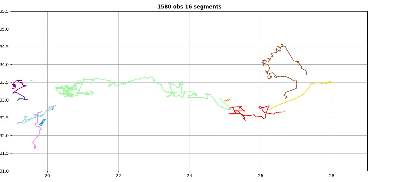
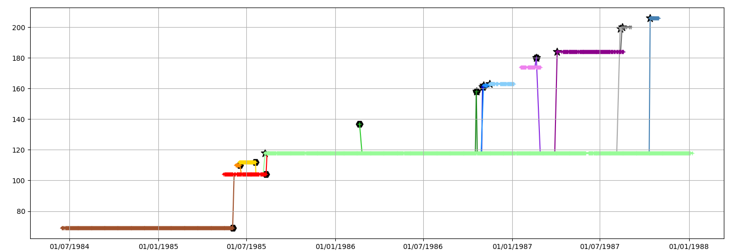
Display the default segmentation

ax = start_axes(n_.infos())
n_.plot(ax, color_cycle=n.COLORS)
update_axes(ax)
fig = plt.figure(figsize=(15, 5))
ax = fig.add_axes([0.04, 0.05, 0.92, 0.92])
ax.xaxis.set_major_formatter(formatter), ax.grid()
_ = n_.display_timeline(ax)

• 
• 

Run a new segmentation

e = n.astype(MyTrackEddiesObservations)
e.obs.sort(order=("track", "time"), kind="stable")
split_matrix = e.split_network(intern=False, window=7)
n_ = NetworkObservations.from_split_network(e, split_matrix)
n_ = n_.relative(get_obs(n_), order=2)
n_.numbering_segment()

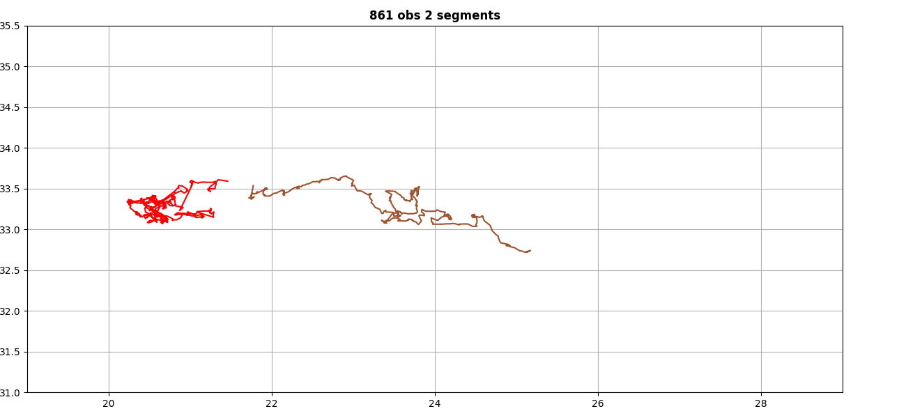
New segmentation

“The oldest wins” method produce a very long segment

ax = start_axes(n_.infos())
n_.plot(ax, color_cycle=n_.COLORS)
update_axes(ax)
fig = plt.figure(figsize=(15, 5))
ax = fig.add_axes([0.04, 0.05, 0.92, 0.92])
ax.xaxis.set_major_formatter(formatter), ax.grid()
_ = n_.display_timeline(ax)

• 
• 

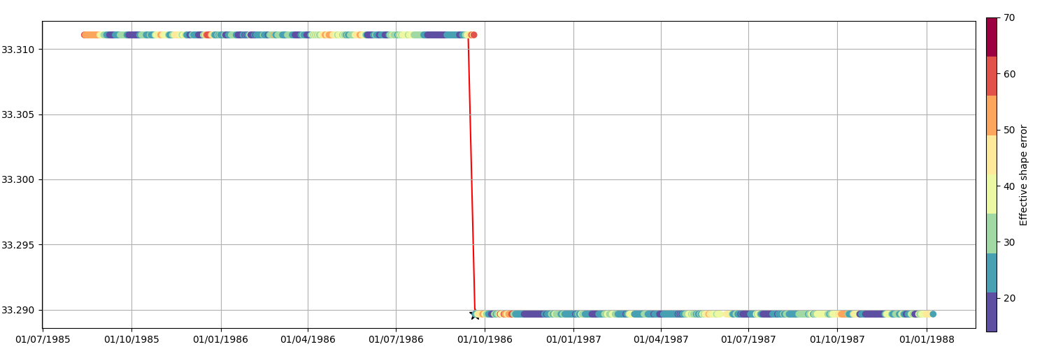
Parameters timeline

kw = dict(s=35, cmap=plt.get_cmap("Spectral_r", 8), zorder=10)
ax = timeline_axes()
n_.median_filter(15, "time", "latitude")
m = n_.scatter_timeline(ax, "shape_error_e", vmin=14, vmax=70, **kw, yfield="lat")
cb = update_axes(ax, m["scatter"])
cb.set_label("Effective shape error")

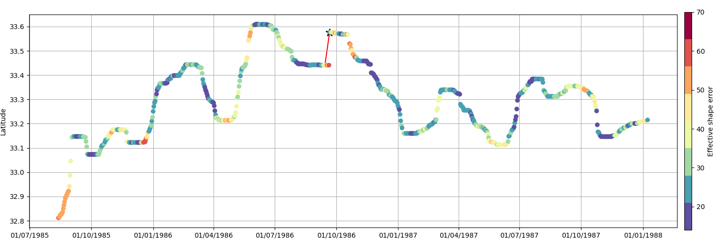
ax = timeline_axes()
n_.median_filter(15, "time", "latitude")
m = n_.scatter_timeline(
    ax, "shape_error_e", vmin=14, vmax=70, **kw, yfield="lat", method="all"
)
cb = update_axes(ax, m["scatter"])
cb.set_label("Effective shape error")
ax.set_ylabel("Latitude")

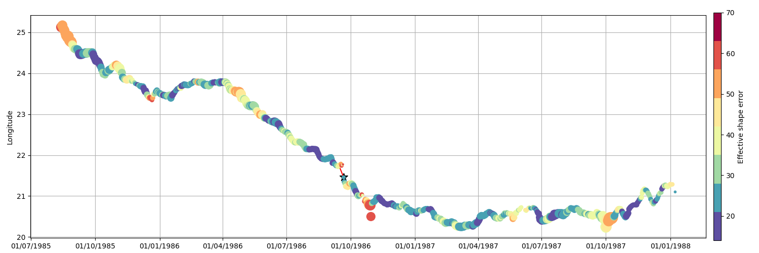
ax = timeline_axes()
n_.median_filter(15, "time", "latitude")
kw["s"] = (n_.radius_e * 1e-3) ** 2 / 30**2 * 20
m = n_.scatter_timeline(
    ax, "shape_error_e", vmin=14, vmax=70, **kw, yfield="lon", method="all"
)
ax.set_ylabel("Longitude")
cb = update_axes(ax, m["scatter"])
cb.set_label("Effective shape error")

• 
• 
• 

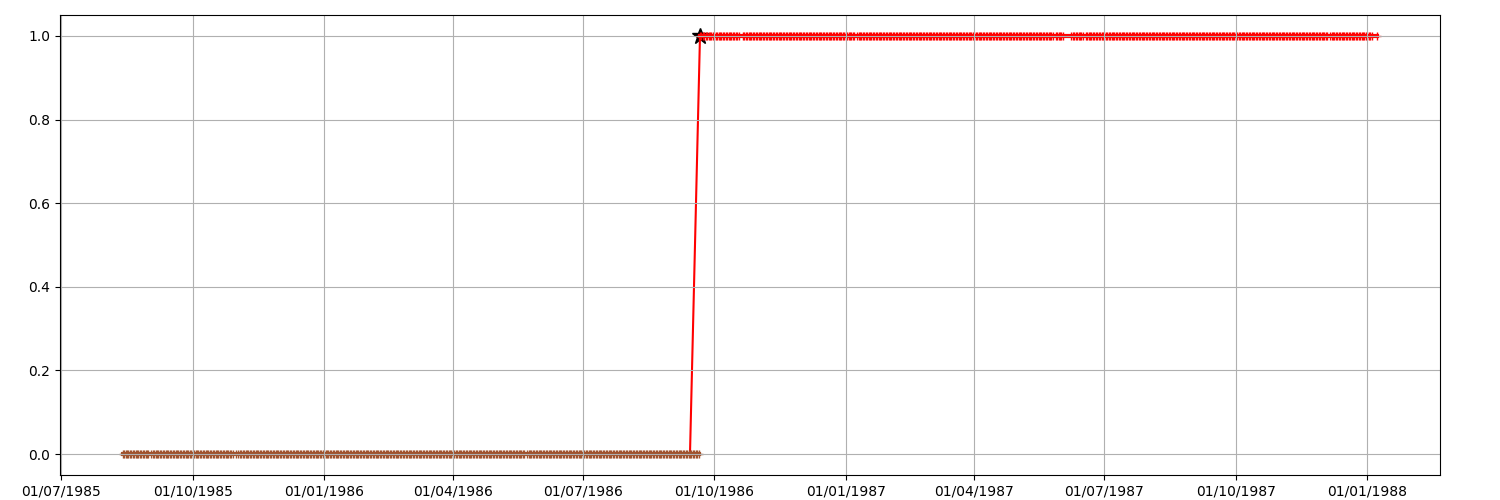
Cost association plot

n_copy = n_.copy()
n_copy.median_filter(2, "time", "next_cost")
for b0, b1 in [
    (datetime(i, 1, 1), datetime(i, 12, 31)) for i in (2004, 2005, 2006, 2007, 2008)
]:
    ref, delta = datetime(1950, 1, 1), 20
    b0_, b1_ = (b0 - ref).days, (b1 - ref).days
    ax = timeline_axes()
    ax.set_xlim(b0_ - delta, b1_ + delta)
    ax.set_ylim(0, 1)
    ax.axvline(b0_, color="k", lw=1.5, ls="--"), ax.axvline(
        b1_, color="k", lw=1.5, ls="--"
    )
    n_copy.display_timeline(ax, field="next_cost", method="all", lw=4, markersize=8)

    n_.display_timeline(ax, field="next_cost", method="all", lw=0.5, markersize=0)

• 
• 
• 
• 
•